Wednesday, May 17, 2023

Video from Arndt-Corden Seminar

Today, I gave a seminar in the Arndt-Corden Department of Economics Seminar Series, titled: "Electricity Markets with Speculative Storage and Stochastic Generation and Demand." We hope to post a working paper soon. In the meantime, here's the video * of my seminar: 


 * Introduction and question time deleted

Tuesday, December 20, 2022

Changes in Authorship, Networks, and Research Topics in Ecosystem Services

I have a new paper, coauthored with Ida Kubiszewski, Bob Costanza, and Luke Concollato, which investigates the development of the field of ecosystem services over the last decade since the founding of the journal Ecosystem Services. This is an open access publication – my first in a so-called hybrid journal. We used the University College London read and publish agreement with Elsevier to publish the paper. ANU now has a similar agreement starting in 2023.

The paper updates Ida and Bob's paper published in 2012: "The authorship structure of ‘‘ecosystem services’’ as a transdisciplinary field of scholarship". In this paper, we update and expand that analysis and compare results with those we found in the previous analysis. We also analyse the influence that the journal Ecosystem Services has had on the field over its first 10 years. We look at which articles have had the most influence on the field (as measured by the number of citations in Ecosystem Services) and on the broader scientific literature (as measured by total citations). We also look at how authorship networks, topics, and the types of journals publishing on the topic have changed. 

Not surprisingly, there has been significant growth in the number of authors (12,795 to 91,051) and number of articles published (4,948 to 33,973) on ecosystem services since 2012. Authorship networks have also expanded significantly, and the patterns of co-authorship have evolved in interesting ways. The most prolific authors are no longer in as tight clusters as they were 10 years ago.

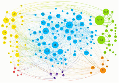
The network chart shows the coauthorship relations among the 163 most prolific authors – those authors who have published more than 30 articles in the field. Colors indicate continent: Yellow = North America, red = South America, blue = Europe, purple – Africa, green = Asia, and orange = Oceania. The greatest number of authors is in Europe and they almost all collaborate with other top authors. Only in Asia and to a lesser degree North America are there top authors who do not collaborate with other top authors.

Costanza et al. (1997) is the most influential article in terms of citations in the journal Ecosystem Services and "Global estimates of the value of ecosystems andtheir services in monetary units" by de Groot et al. (2012) is now the most cited article published in Ecosystem Services.

Ecosystem Services is now the most prolific publisher of articles on ecosystem services among all the journals that have published in the area. There are nine journals that are both on the list of the 20 journals cited most often in Ecosystem Services and on the list of the top 20 journals cited by articles published in Ecosystem Services: Ecosystem Services, Ecological Economics, Ecological Indicators, Science of the Total Environment, Land Use Policy, Journal of Environmental Management, PLoS One, Ecology and Society, and Environmental Science & Policy.

Sunday, December 18, 2022

Annual Review 2022

I've been doing these annual reviews since 2011. They're mainly an exercise for me to see what I accomplished and what I didn't in the previous year. 
 
This was the second year since I have been back living in Canberra in 2007 that I spent the entire year in the Canberra region (extending to the coast) and the second year since 1991 that I didn't fly on a plane. I also haven't been outside of Australasia since 2018. It's pretty hard to travel for any length of time without taking the family and with two small children neither of us feels like traveling anywhere very far. I think we can finally say that the pandemic is over when ANU finally lifted their mask mandates in late October. The university seems pretty dead post-pandemic outside Kambri at lunchtime. Some of our students are still stuck in China etc. but even people who are in Canberra have been reluctant to show up. Graduation week in mid-December showed a flurry of activity.


Kambri

For the first three months of the year, I was supposedly on long service leave (LSL). This might sound good, but actually it is a sacrifice of close to AUD 50k that I would otherwise have been paid out when I retired. I did it to help the university's budget... In return I only taught one course this year. But I ended up agreeing to teach a course that was new to me: IDEC8018 Agricultural and Resource Economics. This turned out to be a huge amount of work in terms of preparation. I started working on the course in February. So, I'm not sure I gained much from my LSL. The main benefit is that I have now managed to move my teaching to Semester 2, which I think is better.  I taught lectures in hybrid mode – an in-person lecture livestreamed on Zoom. Tutorials were split between an in-person and an online tutorial. I think the course went well given it was the first run and there were various hiccups along the way. The teaching evaluations are strong.
 
The main new research I did this year was our paper on confidence intervals for recursive journal impact factors. This research followed up on my 2013 Journal of Economic Literature which computed standard errors and confidence intervals for journal impact factors. Back then, I speculated that confidence intervals could be computed for recursive impact factors and now we've done it. As usual, various collaborative research projects are in progress. Some are mentioned on my research page. I also worked with Ida Kubiszewski and Bob Costanza on a paper on the field of ecosystem services, which we have already published.

I only published two papers with a 2022 date:

Berner A., S. Bruns, A. Moneta, and D. I. Stern (2022) Do energy efficiency improvements reduce energy use? Empirical evidence on the economy-wide rebound effect in Europe and the United States, Energy Economics 110, 105939.

Jafari M., D. I. Stern, and S. B. Bruns (2022) How large is the economy-wide rebound effect in middle income countries? Evidence from Iran, Ecological Economics 193, 107325.

and one with a 2023 date: 

Kubiszewski, I., L. Concollato, R. Costanza, D. I. Stern (2023) Changes in the authorship, networks, and research topics in ecosystem services, Ecosystem Services 101501.

We have one in press paper:

Timilsina, G., Stern, D. I., and D. Das (in press) Physical infrastructure and economic growth, Applied Economics.

Following ANU signing read and publish agreements with Elsevier and Taylor and Francis among others, these will be my first open access articles in hybrid journals.

We only posted one new working paper:

Confidence Intervals for Recursive Journal Impact Factors. June 2022. With Johannes König and Richard Tol.

We have two journal articles under review at the moment. There are a lot of other papers on my to do list, but they range from one we are actively trying to complete, to ones that I haven't really done anything on any time recently and ones that may never happen.

I gave a couple of online conference and seminar presentations. The first was in March in the FEEM Economic Modelling Seminar Series on the topic of Asymmetric Response of Carbon Emissions to Changes in GDP and Negative Oil Market Shocks. The second was a presentation at Enercon 2022, The 3rd International Conference on Energy and Environmental Economics, hosted by the University of the Philippines Los Banos in July. I was asked to give a presentation on the environmental Kuznets curve.

Google Scholar citations exceeded 23,000 with an h-index of 58. I wrote fewer blogposts this year. Eight in total compared to fifteen in 2021. Twitter followers rose from 1650 to almost 1750 over the year. I reviewed 13 journal articles, two tenure or promotion cases, one book proposal, and one grant proposal. I think about one of these per month is about the right number. So, I turn down quite a lot of journal article and some grant review requests. I prioritize journals that I have published in or have been reviewed by recently.

My PhD students Xueting Zhang and Debasish Das continued their research. Suryadeepto Nag has been visiting Crawford to work with me on his master's project, which I am jointly supervising, since late November. We are researching the impact of electrification on development in rural India using Indian survey data.

Looking forward to 2023, a few things can be predicted:

Wednesday, October 19, 2022

What Changed in the World Bank's Adjusted Net Saving Measure?

In August, I showed that using the World Development Indicators' current Adjusted Net Saving (ANS) data there is no relationship between ANS and the share of mining rents in GDP. I now know the main reason why this relationship appeared to change but I don't know yet why the World Bank made the changes that they did. 

In 2006 and earlier, the World Bank measured mineral and energy depletion using mining rents – the difference between mining revenues and the cost of production not including a return to the resource stock. This is based on Hartwick's Rule – resource rents should all be invested in produced capital in order to achieve sustainability. 

In recent years, they have used a different method. First, they estimate the net present value of resource rents (assuming that they remain constant in the future) using a 4% discount rate. Then they divide that amount by the number of years, T, that they assume the resource would last. The ratio of the current rent to this quantity is given by:

So, for example, if the resource has an expected 30 year lifetime then resource depletion is about 58% of current rents. Energy depletion for Saudi Arabia is around 1/3 of reported rents. This would imply that the lifetime of the resource is around 70 years.* This could explain in general why adjusted net saving is now estimated to be much higher for resource rich countries than it used to be.**

What I don't know yet is why they made this change. I haven't been able to find a rationale in the relevant World Bank publications. It is similar to but different from the El-Serafy (1989) method of measuring depletion. According to El-Serafy, the ratio of depletion to rent should be (1/(1+r))^(T+1). For a 30-year life span and a 4% discount rate, this is equal to 30%.

* The notes downloaded with the WDI data say that the lifetime is capped at 25 years. But this isn't mentioned in the relevant reports and makes the gap between rents and depletion harder to explain.

** There are a lot of other issues with assuming that the lifetime of a resource equals the expected lifetime of reserves and that rents will not change over time. There are also apparent inconsistencies between the stated methods and the results...

Thursday, August 11, 2022

Do Mining Economies Save Too Little?

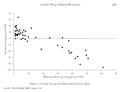
I'm currently teaching Agricultural and Resource Economics for the first time. This week we started covering non-renewable resources focusing on minerals. One of the topics I covered is the resource curse. One of my sources is van der Ploeg's article "Natural Resources: Curse or Blessing?" published in the Journal of Economic Literature in 2011. In the paper, he reproduces this graph from a 2006 World Bank publication that apparently uses 2003 data from the World Development Indicators:

Genuine saving – now known as "adjusted net saving" – is equal to saving minus capital depreciation and various forms of resource depletion with expenditure on education added on. The idea is to measure the net change in all forms of "capital" in an economy. Mineral and energy rents are the pre-tax economic profits of mining. They are supposed to represent the return to the resource stock. The graph tells a clear story: Countries whose GDP depends heavily on mining tend to have negative genuine saving. So, they are not adequately replacing their non-renewable resources with other forms of capital. Van der Ploeg states that this is one of the characteristics of the resource curse.

Preparing for an upcoming tutorial on adjusted net saving and sustainability, I downloaded WDI data for recent years for some mining intensive countries, expecting to show the students how those countries still aren't saving enough. But this wasn't the case. Most of the mining economies had positive adjusted net saving. So, I wondered whether they had improved over time and downloaded the data for all available countries for 2003:


I've added a linear regression line.* There seems to be little relationship between these variables. The correlation coefficient is -0.017. Presumably, this is because of revisions to the data since 2006.

* I dropped countries with zero mining rents from the graph. The three countries at  top right with positive adjusted net saving are Saudi Arabia, Kuwait, and Libya. Oman and then does Democratic Republic of Congo have the next highest levels of mining rents and negative adjusted net savings.

Sunday, August 7, 2022

Trends in RePEc Downloads and Abstract Views

For the first time in a decade, I updated my spreadsheet on downloads and abstract views per person and per item on RePEc.


The downward trends I identified ten years ago have continued, though there was an uptick during the pandemic, which has now dissipated. There was more of an increase in abstract views than in downloads in the pandemic.

Since the end of 2011 both abstract views and downloads per paper have fallen by about 80%. Total papers rose by around 260%, while total downloads fell 38% and total abstract views 27%. 

I'd guess that a mixture of the explanatory factors I suggested last time has continued to be in play.


Thursday, June 2, 2022

Confidence Intervals for Recursive Journal Impact Factors

I have a new working paper coauthored with Johannes König and Richard Tol. It's a follow up to my 2013 paper in the Journal of Economic Literature, where I computed standard errors for simple journal impact factors for all economics journals and tried to evaluate whether the differences between journals were significant.* In the new paper, we develop standard errors and confidence intervals for recursive journal impact factors, which take into account that some citations are more prestigious than others, as well as for the associated ranks of journals. We again apply these methods to the all economics journals included in the Web of Science.

Recursive impact factors include the popular Scimago Journal Rank, or SJR, and Clarivate's Article Influence score. We use Pinski and Narin's invariant method, which has been used in some rankings of economics journals

As simple impact factors are just the mean citations an article published in a journal in a given period receives in a later year, it is easy to compute standard errors for them using the formula for the standard error of the mean. But the vector of recursive impact factors is the positive eigenvector of a matrix and its variance does not have a simple analytical form.

So, we use bootstrapping to estimate the distribution of each impact factor. Taking all 88,928 articles published in 2014-18 in the economics journals included in the Web of Science, we resample from this dataset and compute the vector of recursive impact factors from the new dataset.** Repeating this 1,000 times we pick the 2.5% or 97.5% range of values for each journal to get a 95% confidence interval:

95% confidence intervals of the recursive impact factor, arithmetic scale (left axis) and logarithmic scale (right axis).

The graph repeats the same data twice with different scales so that it's possible to see some detail for both high- and low-ranked journals. Also, notice that while the confidence intervals for the highest ranked journals are quite symmetric, confidence intervals become increasingly asymmetric as we go down the ranks. 

The top ranked journal, the Quarterly Journal of Economics, clearly stands out above all others. The confidence intervals of all other journals overlap with those of other journals and so the ranks of these journals are somewhat uncertain.*** So, next we construct confidence intervals for the journals' ranks.

It turns out that there are a few ways to do this. We could just construct a journal ranking for each iteration of the bootstrap and then derive the distribution of ranks for each individual journal across the 1,000 iterations. Hall and Miller (2009), Xie et al. (2009), and Mogstad et al. (2020) show that this procedure may not be consistent when some of the groups (here journals) being ranked are tied or close to tied. The corrected confidence intervals are generally broader than the naive bootstrap approach.

We compute confidence intervals for ranks using the simple bootstrap, the Xie et al. method, and the Mogstad et al. method:


95% confidence intervals of the rank based on the recursive impact factor. The inner intervals are based on Goldstein’s bootstrap method, the middle intervals use Xie’s correction to the bootstrap, and the outer intervals follow Mogstad’s pairwise comparison.

The simple bootstrap under-estimates the true range of ranks, while it seems that the Mogstad et al. method might be overly conservative. On the other hand, Xie et al.' s approach depends on choosing a couple of "tuning parameters".  

All methods agree that the confidence interval of the rank of the Quarterly Journal of Economics only includes one. Based on the simple bootstrap, the remainder of the "Top-5'' journals are in the top 6 together with the Journal of Finance, while the Xie et al. method and the Mogstad et al. methods generally broaden estimated confidence intervals, particularly for mid-ranking journals. All methods agree that most apparent differences in journal quality are, in fact, mostly insignificant. We think that impact factors, whether simple or recursive should always be published together with confidence intervals.

* The latter exercises were a bit naive. As pointed out by Horrace and Parmeter (2017), we need to account for the issue of multiple comparisons. 

** Previous research on this topic resampled at the journal level, missing most of the variation in citation counts.

*** Overlapping confidence intervals don't neccessarily mean that there is no signficant difference between two means. Goldstein and Harvey (1995) show that the correct confidence intervals for such a test of the difference between two means are narrower than the conventional 95% confidence intervals. On the other hand, for multiple comparisons we would want wider confidence intervals.

Wednesday, January 26, 2022

Typo in Directed Technical Change and the British Industrial Revolution

I hate reading my papers after they're published as there is usually some mistake somewhere. Unfortunately, I have to read them to do more research. I just found a typo in our 2021 paper in JAERE. Equation (8) should look like this:


In the published paper, there is a missing Gamma in the second term. 

I also noticed a couple of issues in the text of "Energy quality" published in Ecological Economics in 2010. One is in the introduction and is debatable: "Fuel and energy quality is not neccessarily fixed". This should be or instead of and or are instead of is. But it really isn't important. Then on p1475 we have "How does these measures". Again, not important.

Of course, the error in JAERE is not very important as the third term above is correct in the published paper.

Thursday, December 30, 2021

Annual Review 2021

I've been doing these annual reviews since 2011. They're mainly an exercise for me to see what I accomplished and what I didn't in the previous year. 

This was the first year since I have been back living in Canberra in 2007 that I spent the entire year in the Canberra region. In fact, it is the first year since 1991 that I didn't fly on a plane. It's not that unusual for me not to leave my country for a year. I didn't travel outside of Australia in 2019. This year, with a two year old and random snap lockdowns happening in the first part of the year, we were not in the mood to travel anywhere overnight even when it was possible. Then from mid-August came the second Canberra lockdown for 2 plus months (the first was during the first wave of the pandemic in March-May 2020). Luckily I was able to take Isaac (the two year old) to daycare throughout the lockdown, but we had to help homeschool Noah (5 years old). I was impressed how well the school organized things. Before Omicron came along, things had returned almost to normality in Canberra. We still needed to wear masks at the daycare and on the bus and needed to check in sometimes at stores etc. The university has been dragging its feet on the return to campus, but the faculty office areas in the Crawford Building have sometimes been even a little bit busy. In the last week of the year, I finally travelled out of Canberra with my family to go on holidays on the NSW South Coast.


While we've been away from Canberra the number of COVID-19 cases has been growing radically. Almost everyone here is vaccinated and Omicron seems less severe, so it's unclear what this will mean for university activity in 2022. They were planning a more or less complete return to on campus teaching, but who knows now...
 
In Semester 1 (from February to June), I again taught environmental economics and the masters research essay course. But this is the last time I will be teaching them. More about that in the 2022 predictions, below. We taught in hybrid mode. In the environmental economics class there was a joint online lecture for online and on campus students and then separate tutorials for the two groups. It turned out that very few people came to the in person tutorial. Often I had only one student. But this session was much better in my opinion than either of the online sessions. The masters research essay class had separate online and in-person classes.
 
I was awarded a Francqui Chair at the University of Hasselt in Belgium for the 2020-21 academic year. The main duty of the position was to give ten hours of lectures. Of course, I didn't actually travel to Belgium and so I gave five online lectures. You can see the videos and read some commentary on my blog.

 
I can't really think of anything notable to say about my research activity this year. It's mostly been a story of completing existing projects. We finally wrapped up our ARC DP12 project (yes, funding started in 2012 and we submitted the proposal in 2011) with the publication of our paper on the Industrial Revolution in JAERE.

I started working on several new ideas in the second half of the year but they don't seem to be going anywhere or have already been abandoned. The exception is our asymmetry paper, which we started thinking about right at the end of 2020 and now is under review.

We published five papers with a 2021 date:

Stern D. I., J. C. V. Pezzey, and Y. Lu (2021) Directed technical change and the British Industrial Revolution, Journal of the Association of Environmental and Resource Economists 8(6), 1079-1114.

Saunders H., J. Roy, I. Azevedo, D. Chakravarty, S. Dasgupta, S. de la rue du Can, A. Druckman, R. Fouquet, M. Grubb, B.-Q. Lin, R. Lowe, R. Madlener, D. McCoy, L. Mundaca, T. Oreszczyn, S. Sorrell, D. I. Stern, K. Tanaka, and T. Wei (2021) Energy efficiency: What has research delivered in the last 40 years? Annual Review of Environment and Resources 46, 135-165.

Dressel B. and D. I. Stern (2021) Research at public policy schools in the Asia-Pacific region ranked, Asia and the Pacific Policy Studies 8(1), 151-166.

Stern D. I. and R. S. J. Tol (2021) Depth and breadth relevance in citation metrics, Economic Inquiry 59(3), 961-977.

Bruns S. B., A. Moneta, and D. I. Stern (2021) Estimating the economy-wide rebound effect using empirically identified structural vector autoregressions, Energy Economics 97, 105158.

and one paper with a 2022 date:

Jafari M., D. I. Stern, and S. B. Bruns (2022) How large is the economy-wide rebound effect in middle income countries? Evidence from Iran, Ecological Economics 193, 107325.

We posted four new working papers:

How Much Does Physical Infrastructure Contribute to Economic Growth? An Empirical Analysis
December 2021. With Govinda Timilsina and Debasish Das.

Asymmetric Response of Carbon Emissions to Recessions and Expansions and Oil Market Shocks
October 2021. With Xueting Jiang.

How Large is the Economy-Wide Rebound Effect in Middle Income Countries? Evidence from Iran
August 2021. With Mahboubeh Jafari and Stephan Bruns.

Do Energy Efficiency Improvements Reduce Energy Use? Empirical Evidence on the Economy-Wide Rebound Effect in Europe and the United States
May 2021. With Anne Berner, Stephan Bruns, and Alessio Moneta.

We have three papers under review at the moment (one – the Europe rebound one – is a resubmission). There are twelve other papers on my to do list, but they range from one we are actively trying to complete, to ones that I haven't really done anything on any time recently.

Google Scholar citations exceeded 21,000 with an h-index of 55. I wrote more blogposts this year. Fifteen in total compared to ten in 2020. Twitter followers rose from 1500 to more than 1650 over the year. I did 3 external assessments of people for promotion or tenure for universities in Australia, Hong Kong, and Germany. Fewer than last year. I only did 11 reviews for journals. I used to do around double this three or more years back. And I reviewed a bunch of papers for EAERE, a proposal for the ARC, as well as giving people feedback on their papers etc.

My PhD student Xueting Zhang completed her first research year. She has made a lot of progress, with three papers at various stages of completion. My other student Debasish Das continued his work on prepaid metering and a lot of other stuff, some of which you can check out on his Google Scholar profile.

Looking forward to 2022, a few things can be predicted: 

  • I will be teaching a new course (for me) in the second semester: Agricultural and Resource Economics. It is going to take a lot of work to prepare this course. 
  • As a result, I won't be teaching in the first semester. Officially, I will be on long service leave, which is how I got my teaching reduced to one course for the year. But I will need to work hard on both the course and research right from the start of the year. OK, I'm feeling like taking 4th January off :) The university has encouraged us to take long service leave to help the budget situation. Taking the leave releases money from the account where it has been set aside and they don't need to pay my salary from the recurrent budget.
  • I'm hoping we will get our paper on the rebound effect in Europe accepted very soon.
  • I probably will stay in Australia for this year too. Anyway, I haven't set up any international travel at this stage.

Tuesday, December 21, 2021

Estimating the Effect of Physical Infrastructure on Economic Growth

I have a new working paper coauthored with Govinda Timilsina of the World Bank and my PhD student Debasish Das. It is a panel data study of the effect of various forms of infrastructure on the level of GDP. 

Compared to existing studies, we use more recent data, include new types of infrastructure such as mobile phones, and provide separate estimates for developing and developed countries. We find larger effects than most previous studies. We also find that infrastructure has a larger effect in more recent years (1992-2017) than in earlier years (1970-1991), and the effects of infrastructure are higher in developing economies than in industrialized economies. The long-run effects seem to be much larger than the initial impact. We also tried to estimate the effect of infrastructure on the rate of economic growth. Controlling for the initial level of GDP per worker we found a null result. So, we can't say that having more infrastructure means a more rapid rate of economic growth.

Getting good quality data that is comparable across countries is really a problem in this area of research. Many types of infrastructure only have data available for a few years. The ones that have more panel-like data often suffer from differences in definition across countries – such as what is a road or a motorway – or unexplained jumps in individual countries. So, our results are subject to a lot of measurement error.

Our main analysis uses data on five types of infrastructure – roads, railways, electric generation capacity, fixed line telephones, and mobile telephones*:

Following some previous research, we aggregate the individual types of infrastructure using principal component analysis. We use two principal components. One factor seems to be related to transport infrastructure and the other to electricity and telecommunications. Still, we can recover estimates of the effect of each individual type of infrastructure.

Also following some previous research, we use the Pooled Mean Group estimator to estimate a dynamic panel regression model. This allows us to test for the weak exogeneity of the explanatory variables, allowing us to give the results a somewhat causal interpretation.

The table shows the percentage change in GDP per worker for a 1% change in each infrastructure type. Getting standard errors for these estimates would be rather tricky.** Interestingly, the PMG estimates are mostly much larger than the static fixed effects estimates. Static fixed effects can be expected to converge to a short-run estimate of the effects while PMG should be a better estimate of long-run effects. Fixed effects also tends to inflate the effects of measurement error

Maybe the most innovative thing in the paper is that we plot the impulse response functions of GDP with respect to a 1% increase in each of the two main types of infrastructure:

PC1 is electricity and communications and PC2 transport infrastructure.*** Long-run effects of infrastructure are much larger than the short-run effects. In the short run, transport infrastructure even has a negative impact.

* Note that the graphs show the country means of these variables, while we actually use the deviations from those means over time in each country

** We only estimate the GDP-infrastructure relationship, but I think we would need time series models for each of the explanatory variables in order to sample from those models' residuals in a bootstrapping procedure. Bootstrapping is needed because we first carry out the principal components analysis and then estimate the PMG model in a second stage. These elasticities are combinations of the parameters from those two models.

*** We could get a confidence interval for these impulse response functions if we assume that the explanatory variables in the PMG model are deterministic as this analysis assumes...


Thursday, October 21, 2021

The Environmental Kuznets Curve: 2021 Edition

The second encyclopedia chapter. First one is here.

Introduction 

The environmental Kuznets curve (EKC) is a hypothesized relationship between various indicators of environmental degradation and countries’ gross domestic product (GDP) per capita. In the early stages of a country’s economic development, environmental impacts and pollution increase, but beyond some level of GDP per capita (which will vary for different environmental impacts) economic growth leads to environmental improvement. This implies that environmental impacts or emissions per capita are an inverted U-shaped function of GDP per capita, whose parameters can be statistically estimated. Figure 1 shows a very early example of an EKC. A large number of studies have estimated such curves for a wide variety of environmental impacts ranging from threatened species to nitrogen fertilizers, though atmospheric pollutants such as sulfur dioxide and carbon dioxide have been investigated most. Panayotou (1993) was the first to call this relationship the EKC, where Kuznets refers to the similar relationship between income inequality and economic development proposed by Nobel Laureate Simon Kuznets and known as the Kuznets curve. The EKC can be seen as an empirical version of the interpretation of sustainable development as the idea that development is not necessarily damaging to the environment and, also that poverty reduction is essential to protect the environment (World Commission on Environment and Development, 1987).

Figure 1. An Environmental Kuznets Curve 

The EKC has been the dominant approach among economists to modeling ambient pollution concentrations and aggregate emissions since Grossman and Krueger (1991) introduced it in an analysis of the potential environmental effects of the North American Free Trade Agreement. The EKC also featured prominently in the 1992 World Development Report published by the World Bank and has since become very popular in policy and academic circles and is even found in introductory economics textbooks. 

Critique 

Despite this, the EKC was criticized almost from its beginning on empirical and policy grounds, and debate continues. It is undoubtedly true that some dimensions of environmental quality have improved in developed countries at the same time that they have become richer. City air and rivers in these countries have become cleaner since the mid-20th Century and, in some countries, forests have expanded. Emissions of some pollutants such as sulfur dioxide have clearly declined in most developed countries in recent decades. But there is more mixed evidence for other pollutants such as carbon dioxide. Carbon emissions have fallen in the last 40 years in some developed countries such as the United Kingdom or Sweden, while they have increased in others such as Australia or Japan. There is also evidence that emerging countries take action to reduce severe pollution. For example, Japan cut sulfur dioxide emissions in the early 1970s following a rapid increase in pollution when its income was still below that of the developed countries (Stern, 2005) and China has also acted to reduce sulfur emissions in recent years. As further studies were conducted and better data accumulated, many of the econometric studies that supported the EKC were found to be statistically fragile. 

Initially, many understood the EKC to imply that the best way for developing countries to improve their environment was to get rich (e.g. Beckermann, 1992). This alarmed others (e.g. Arrow et al., 1995), as while this might address some issues like deforestation or local air pollution, it would likely exacerbate other environmental problems such as climate change. Even if there is an EKC for per capita impacts, environmental impacts would increase for a very long time if the majority of the population is on the rising part of the curve and/or the population is also growing (Stern et al., 1996). 

Explanations 

The existence of an EKC can be explained either in terms of deep determinants such as technology and preferences or in terms of scale, composition, and technique effects, also known as “proximate factors”. Scale refers to the effect of an increase in the size of the economy, holding the other effects constant, and should increase environmental impacts. The composition and technique effects must outweigh this scale effect for pollution or other environmental impacts to fall in a growing economy. The composition effect refers to the economy’s mix of different industries and products, which differ in pollution intensities. Finally, the technique effect refers to the remaining change in pollution intensity. This will include contributions from changes in the input mix, for example substituting natural gas for coal; changes in productivity that result in less use, ceteris paribus, of polluting inputs per unit of output; and pollution control technologies that result in less pollutant being emitted per unit of polluting input. 

Over the course of economic development, the mix of energy sources and economic outputs tends to evolve in predictable ways. Economies start out mostly agricultural and the share of industry in economic activity first rises and then falls as the share of agriculture declines and the share of services increases. We might expect the impacts associated with agriculture, such as deforestation, to decline, and naively expect the impacts associated with industry, such as pollution, would first rise and then fall. However, the absolute size of industry rarely does decline, and it is improvement in productivity in industry, a shift to cleaner energy sources, such as natural gas and hydro-electricity, and pollution control that eventually reduce some industrial emissions. On the other hand, offshoring of pollution probably plays only a small role in cutting emissions in developed economies (Kander et al., 2015). 

Static theoretical economic models of deep determinants, that do not try to also model the economic growth process, can be summarized in terms of two parameters: The elasticity of substitution between dirty and clean inputs, which summarizes how difficult it is to cut pollution; and the elasticity of the marginal utility of consumption with respect to consumption, which summarizes how hard it is to increase consumer well-being with more consumption (Pasten and Figeroa, 2012). It is usually assumed that these consumer preferences are translated into policy action. Pollution is then more likely to increase as the economy expands, the harder it is to substitute other inputs for polluting ones and the easier it is to increase consumer well-being with more consumption. If these parameters are constant, then either pollution rises or falls with economic growth. Only if they change over time will pollution first rise and then fall. The various theoretical models can be classified as ones where the EKC is driven by changes in the elasticity of substitution as the economy grows or models where the EKC is primarily driven by changes in the elasticity of marginal utility. 

Dynamic models that model the economic growth process alongside changes in pollution are harder to classify. The Green Solow Model developed by Brock and Taylor (2010) explains changes in pollution as a result of the competing effects of economic growth and a constant rate of improvement in pollution control. Fast growing middle-income countries, such as China, then having rising pollution, and slower growing developed economies, falling pollution. An alternative model developed by Ordás Criado et al. (2011) also suggests that pollution rises faster in faster growing economies but that there is also convergence so that countries with higher levels of pollution are more likely to reduce pollution faster than countries with low levels of pollution. 

Recent Empirical Research 

Recent empirical research builds on these dynamic models to paint a subtler picture than early EKC studies did (Stern, 2017). We can distinguish between the impact of economic growth on the environment and the effect of the level of GDP per capita, irrespective of whether an economy is growing or not, on reducing environmental impacts. We can also distinguish between the effects of economic growth and the simple passage of time. Economic growth usually increases environmental impacts, but the size of this effect varies across impacts and the impact of growth often declines as countries get richer. However, richer countries are often likely to make more rapid progress in reducing environmental impacts. In econometric terms, the time effect – the change in emissions if economic growth is zero – may be higher in richer countries. Rapid growth in middle-income countries, such as China or India, is more likely to overwhelm the time effect in those countries as suggested by Brock and Taylor (2010).

Finally, there is often convergence among countries, so that those that have relatively high levels of impacts reduce them faster or increase them slower than countries with low levels of impacts. These combined effects explain more of the variation in pollution emissions or concentrations than either the classic EKC model or models that assume that either only convergence or growth effects alone are important. Therefore, while being rich means a country might do more to clean up its environment, getting rich is likely to be environmentally damaging. 

References 

Arrow, K., Bolin, B., Costanza, R., Dasgupta, P., Folke, C., Holling, C. S., Jansson, B.-O., Levin, S., Mailer, K.-G., Perrings, C., Pimental, D., 1995. Economic growth, carrying capacity, and the environment. Science 268, 520–521. 

Beckermann, W., 1992. Economic growth and the environment: whose growth? Whose environment? World Development 20, 481–496. 

Brock, W. A.,Taylor, M. S., 2010. The green Solow model. Journal of Economic Growth 15, 127–153. 

Grossman, G. M., Krueger, A. B., 1991. Environmental impacts of a North American Free Trade Agreement. NBER Working Papers 3914. 

Kander, A., Jiborn, M., Moran, D. D., Wiedmann T. O., 2015. National greenhouse-gas accounting for effective climate policy on international trade. Nature Climate Change 5, 431–435. 

Ordás Criado, C., Valente, S., Stengos, T., 2011. Growth and pollution convergence: Theory and evidence. Journal of Environmental Economics and Management 62, 199–214. 

Panayotou, T., 1993. Empirical tests and policy analysis of environmental degradation at different stages of economic development. Working Paper, Technology and Employment Programme, International Labour Office, Geneva, WP238. 

Pasten, R., Figueroa, E., 2012. The environmental Kuznets curve: A survey of the theoretical literature. International Review of Environmental and Resource Economics 6, 195–224. 

Stern, D. I., 2005. Beyond the environmental Kuznets curve: Diffusion of sulfur-emissions-abating technology. Journal of Environment and Development 14(1), 101–124. 

Stern, D. I., 2017. The environmental Kuznets curve after 25 years. Journal of Bioeconomics 19, 7–28.

Stern, D. I., Common, M. S., Barbier, E. B., 1996. Economic growth and environmental degradation: the environmental Kuznets curve and sustainable development. World Development 24, 1151–1160. 

World Commission on Environment and Development, 1987. Our Common Future. Oxford: Oxford University Press.  

Energy and Development

The first of two book chapters for Elgar encyclopedias I recently wrote.

What is the Role of Energy in Economic Activity?

The economic system must operate within the constraints determined by the laws of physics and human knowledge of technology. Production, including household production, requires energy to carry out work to convert materials into desired products and to transport raw materials, goods, and people. The second law of thermodynamics implies that energy cannot be recycled and that there are limits to how much energy efficiency can be improved. Therefore, energy is an essential factor of production, and continuous supplies of energy are needed to maintain existing levels of economic activity as well as to grow and develop the economy (Stern, 1997). The first law of thermodynamics states that energy cannot be created and so energy (and matter) must be extracted from the environment. Also, energy must be invested in order to capture useful energy (Hall et al., 1986). Before the Industrial Revolution, economies depended on energy from agricultural crops and wood as well as a smaller amount of wind and waterpower, all of which are directly dependent on the sun (Kander et al., 2015). This is still largely the case in the rural areas of the least developed countries. While solar energy is abundant and inexhaustible, it is very diffuse compared to concentrated fossil fuels. This is why the shift to fossil fuels in the Industrial Revolution relaxed the constraints on energy supply and, therefore, on production and growth (Wrigley, 1988).

How Does Energy Use Change with Economic Development?

Figure 1 shows that energy use per capita increases with GDP per capita, so that richer countries tend to use more energy per person than poorer countries. The slope of the logarithmic regression line implies that a 1% increase in income per capita is associated with a 0.8% increase in energy use per capita. As a result, energy intensity – energy used per dollar of GDP – is on average lower in higher income countries. These relationships have been very stable over the last several decades (Csereklyei et al., 2016). Energy intensity in today’s middle-income countries is similar to that in today’s developed countries when they were at the same income level (van Benthem, 2015).

Figure 1. GDP and Energy Use per Capita 2018

Energy intensity has also converged across countries over time, so that countries that were more energy intensive in the 1970s tended to reduce their energy intensity by more than less energy intensive countries, and the least energy intensive countries often increased in energy intensity. Though data are limited to fewer and fewer countries as we go back further in time, these relationships also appear to hold over the last two centuries – energy use increased, energy intensity declined globally, and countries converged in energy intensity (Csereklyei et al., 2016). Though data is even more limited, it seems that the share of energy consumption expenditure and production costs also declines as countries develop (Csereklyei et al., 2016; Burke et al., 2018).

The mix of fuels used changes over the course of economic development. Figure 2 shows the average mix of energy sources in each of five groups of countries ordered by income per capita in 2018. In the lowest income countries in the sample (approximately below $5,000 per capita in 2017 purchasing power parity adjusted dollars), traditional use of biomass such as wood and agricultural waste dominates and oil use for transportation as well as electricity generation and other uses is the second most important energy source. As we move to richer countries, the relative role of biomass declines radically, and first oil and then natural gas and primary electricity increase in importance. Note that biomass use per capita in the richest quintile (above $40,000 per capita) is actually greater than in the lowest quintile, as total energy use increases with income. The ways in which this biomass is used will of course be quite different. Higher quality fuels are those that provide more economic value per joule of energy content by being converted more efficiently, being more flexible or convenient to use, and by producing less pollution. We would expect that lower income households would be more willing to tolerate the inconvenience and pollution caused by using lower quality fuels to produce energy services. So as household income increases, we would expect households to gradually ascend an “energy ladder” by consuming higher quality fuels and more total energy. Recent studies often find a more ambiguous picture where multiple fuels are used simultaneously as modern fuels are added to the use of traditional fuels (Gregory and Stern, 2014). 

Figure 2. Fuel Mix and Development 2018


In 2016, approximately one billion people remained without access to electricity at home (International Energy Agency, 2017). Around 85% of these people lived in rural areas. There has been rapid progress in electrification in recent years with both grid expansion and the spread of off-grid systems (Burke et al., 2018; Lee et al., 2020). Due to the complexity and costs of electricity-sector management and constrained and weak institutions, power supply is usually less reliable in developing countries than in developed countries (Figure 3) and electricity theft is also more common (Burke et al., 2018). Best and Burke (2017) found that countries with higher levels of government effectiveness have achieved greater progress in providing access to reliable electricity. Industry and other electricity consumers, therefore, often rely on self-generation of electricity, but this is a costly solution (Fingleton-Smith, 2020). 

 Figure 3. Electricity Reliability and Development 2017


Does Energy Use Drive Economic Growth?

Economic growth refers to the process that results in increasing GDP per capita over time while development refers to a broader range of indicators including health, education, and other dimensions of human welfare. However, GDP per capita is highly, although not perfectly, correlated with broader development measures (Jones and Klenow, 2016) and so it is worth considering what the role of energy is in economic growth.

Mainstream economic growth models largely ignore the role of energy in economic growth and focus on technological change as the long-run driver of growth. On the other hand, there is a resource economics literature that investigates whether limited energy or other resources could constrain growth. By contrast, many ecological economists believe that energy plays the central role in driving growth and point to the switch traditional energy sources to fossil fuels as the cause of the industrial revolution (Stern, 2011). 

To reconcile these opposing views, Stern and Kander (2012) modified Solow’s neoclassical growth model (Solow, 1956) by adding an energy input that has low substitutability with capital and labor. Their model also breaks down technological change into those innovations that directly increase the productivity of energy– energy-augmenting technical change and those that increase the productivity of labor – labor-augmenting technical change. In this model, when energy is superabundant the level of the capital stock and output are determined by the same functions of the same factors as in the Solow model. But when energy is relatively scarce, the size of the capital stock and the level of output depends on the level of energy supply and the level of energy-augmenting technology. Therefore, in the pre-industrial era and possibly when energy was scarce – and possibly in developing countries today – the level of output was determined by the supply of energy and the level of energy augmenting technology. Until the industrial revolution, output per capita was generally low and economic growth was not sustained (Maddison, 2001). After the industrial revolution, as energy became more and more abundant, the long-run behavior of the model economy becomes more and more like the Solow growth model. If this model is a reasonable representation of reality, then mainstream economists are not so wrong to ignore the role of energy in economic growth in developed economies where energy is abundant, but their models have limited applicability to both earlier historical periods and possibly to today’s developing countries. McCulloch and Zileviciute (2017) find that electricity is often cited as a binding constraint on growth in the World Bank’s enterprise surveys. Energy is expensive relative to wages in developing countries. The price of oil is set globally, and the share of electricity in costs or expenditures can be very high in middle income countries (Burke et al., 2018).

Electricity and Development

Access to energy and electricity, in particular, is a key priority for policymakers and donors in low-income countries. For example, the United Nations’ Sustainable Development Goal 7 targets universal access to modern energy by 2030. Electrification can allow poor households to have easy access to lighting for evening chores or studying and power for phone charging and for a range of new small business activities, both on and off the farm (Lee et al., 2020). Electricity access allows a reallocation of household time, especially for women, away from obtaining energy, for example by collecting firewood, and towards more productive activities. Electricity could also provide health benefits by allowing deeper wells, refrigeration, reduced exposure to smoke etc. (Toman and Jemelkova, 2003).

The micro-level effect of electrification is a growing area of empirical research (Lee et al., 2020). While micro studies typically suggest positive impacts of electrification on income and other development outcomes, more recent quasi-experimental approaches such as randomized controlled trials typically find a smaller impact for electrification than earlier studies did (Lee et al., 2020). Estimates of the effect of electricity infrastructure on economic growth are typically small. One of the best studies (Calderón et al., 2015) estimates the elasticity of GDP with respect to electricity generation capacity as 0.03 (Burke et al., 2018).

Lee et al. (2020) argue that providing poor households with access to electricity alone is not enough to improve economic and noneconomic outcomes in a meaningful way. Complementary inputs are needed, which will accumulate very slowly. Imagination and role models are also important in understanding how to exploit electricity to develop businesses (Fingleton-Smith, 2020). When electricity becomes available in rural areas of sub-Saharan Africa, it is often not used to power agricultural or other productive activities (Bernard, 2012). Institutions are also vital for attaining broad-based benefits from electricity in developing countries. Many developing countries have reformed their electricity sectors during the last few decades, mostly towards market liberalization and corporatization. These efforts have only been partially successful in promoting efficient pricing and greater electricity access (Jamasb et al., 2017). Studies assessing the economic effects of these reforms are scarce. The effects on economic growth seem positive, while the effects on poverty are mixed (Jamasb et al., 2017). In this context, technology transfer and development finance will be critical for increasing the use of electricity in developing countries (Madlener, 2009).

Burke et al. (2018) examined electrification success stories - countries that, from a low level of economic development, have now achieved near-universal electricity access as well as relatively high levels of electricity use. These countries are South Korea, China, Thailand, Vietnam, Egypt, and Paraguay. The first four are well-known development success stories too. Paraguay has abundant hydroelectricity and both Paraguay and Egypt have had relatively strong economic growth. Egypt has been less successful in providing a reliable electricity supply. The most successful countries in increasing access in Sub-Saharan Africa have been South Africa and Ghana, which both suffer from unreliable electricity, which constrains economic activity.

References

Bernard, T., 2012. Impact analysis of rural electrification projects in Sub-Saharan Africa. World Bank Research Observer 27(1): 33–51.

Best, R., and P. J. Burke, 2017. The importance of government effectiveness for transitions toward greater electrification in developing countries. Energies 10(9): 1247.

Burke P. J., D. I. Stern, and S. B. Bruns, 2018. The impact of electricity on economic development: a macroeconomic perspective. International Review of Environmental and Resource Economics 12(1): 85–127.

Calderón, C., E. Moral-Benito, and L. Servén, 2015. Is infrastructure capital productive? A dynamic heterogeneous approach. Journal of Applied Econometrics 30: 177–198.

Csereklyei Z., M. d. M. Rubio Varas, and D. I. Stern, 2016. Energy and economic growth: The stylized facts. Energy Journal 37(2): 223–255.

Fingleton-Smith, E., 2020. Blinded by the light: The need to nuance our expectations of how modern energy will increase productivity for the poor in Kenya. Energy Research & Social Science 70: 101731.

Gregory, J. and D. I. Stern, 2014. Fuel choices in rural Maharashtra. Biomass and Bioenergy 70: 302–314.

Hall, C. A. S., C. J. Cleveland, and R. K. Kaufmann, 1986. Energy and Resource Quality: The Ecology of the Economic Process. New York: Wiley Interscience.

International Energy Agency, 2017. Energy Access Outlook 2017: From Poverty to Prosperity. World Energy Outlook Special Report.

Jamasb, T., R. Nepal, and G. R. Timilsina, 2017. A quarter century effort yet to come of age: a survey of electricity sector reform in developing countries. Energy Journal 38(3): 195–234.

Jones, C. I., and P. J. Klenow. 2016. Beyond GDP? Welfare across countries and time. American Economic Review 106(9): 2426–2457.

Kander, A., P. Malanima, and P. Warde, 2014. Power to the People: Energy in Europe over the Last Five Centuries. Princeton University Press.

Lee, K., E. Miguel, and C. Wolfram, 2020. Does household electrification supercharge economic development? Journal of Economic Perspectives 34(1): 122–144.

Maddison, A., 2001. The World Economy: A Millennial Perspective. Paris: OECD.

Madlener, R., 2009. The economics of energy in developing countries. In: L. C. Hunt and J. Evans (eds.), International Handbook on the Economics of Energy, Edward Elgar.

McCulloch, N., and D. Zileviciute, 2017. Is electricity supply a binding constraint to economic growth in developing countries? EEG State-of-Knowledge Paper Series 1.3.

Solow, R. M., 1956. A contribution to the theory of economic growth. Quarterly Journal of Economics 70: 65–94.

Stern, D. I., 1997. Limits to substitution and irreversibility in production and consumption: a neoclassical interpretation of ecological economics. Ecological Economics 21: 197–215.

Stern, D. I., 2011. The role of energy in economic growth. Annals of the New York Academy of Sciences 1219: 26–51.

Stern, D. I., and A. Kander, 2012. The role of energy in the industrial revolution and modern economic growth. Energy Journal 33(3): 125–152.

Toman, M. A., and B. Jemelkova, 2003. Energy and economic development: An assessment of the state of knowledge. Energy Journal 24(4): 93–112.

van Benthem, A. A., 2015. Energy leapfrogging. Journal of the Association of Environmental and Resource Economists 2(1): 93–132.

Wrigley, E. A., 1988. Continuity, Chance, and Change: The Character of the Industrial Revolution in England. Cambridge: Cambridge University Press.

Wednesday, October 20, 2021

Our COVID-19 Paper

Publishing papers on COVID-19 is very popular: 

and we couldn't resist joining the bandwagon. Late last year, Xueting Jiang, my PhD student, and I did a quick literature survey to identify a gap. Though there was a lot of research on how pollution emissions evolved over the course of the pandemic and recession, there was little putting that into the historical context of past recessions. Last year, I worked with Kate Martin, a masters student, on the relationship between carbon emissions and economic activity over the business cycle. We decided to extend that analysis. 

Our new paper uses U.S. monthly data from January 1973 to December 2020. We look at how the relationship between carbon emissions and GDP varies between recessions and expansions, but we also look at individual recessions and how emissions from different sectors vary over the business cycle. 

Like Sheldon and others, we find that, in general, the emissions-GDP elasticity is greater in recessions than in expansions, but we find that this is largely because of sharp falls in emissions associated with negative oil market shocks. The 1973-5, 1980, and 1990-1 recessions were associated with negative oil supply shocks. In 2020, there was instead a negative oil demand shock due to the pandemic. These recessions have emissions-GDP elasticities that are significantly larger than the elasticity in expansions. The elasticities in the 1981-2, 2001, and 2008-9 recessions are no larger than in expansions.

The graph shows NBER recessions in light blue stripes and nominal and real oil prices. The big spike in oil prices in 2008 came at the end of an extended increase associated with rising demand for oil. Of course, supply was constrained during this period but there wasn't a sudden supply crisis. In 1981-82 the price of oil was already falling when the recession started and it is usually regarded as having been caused by the Federal Reserve under Paul Volcker dramatically raising interest rates.

When we regress the growth of sectoral carbon emissions on the growth of national GDP, we find that the asymmetry is present in the industrial and particularly in the transport sector, which are the two largest users of oil in the US economy, using 28% and 66% of the total, respectively.

When we control for oil use, the asymmetries disappear. 

So, though the cause of the COVID-19 recession was unusual the carbon emissions outcome was similar to past recessions associated with oil crises. More importantly, we learned something new about what happens to emissions in recessions, at least in the US.


Tuesday, October 12, 2021

How Large is the Economy-Wide Rebound Effect in Middle Income Countries? Evidence from Iran


We have a new working paper in our rebound effect series. Previous papers reviewed the literature on the economy-wide rebound effect, estimated the economy-wide rebound effect for the United States, and estimated it for some European countries (as well as the United States). The new paper is about Iran. This is a middle income country with a resource intensive and quite regulated economy. Is it a lot different to the developed economies we have already looked at?

The rebound effect is large in Iran too. A major difference between Iran and the developed economies is that energy intensity has been rising in Iran:


Total energy use tripled from 1988 to 2017, which is the sample period used in our econometric analysis (quarterly data):


The econometric model is the same as that used in the US paper that is now published in Energy Economics, except we only use the distance covariance method for the independent component analysis in this paper. The next figure shows the estimated impulse response functions of energy, GDP, and the price of energy to energy efficiency, GDP, and price shocks:

The top left panel shows the rebound effect. Initially, there is a large drop in energy use, but this diminishes over time. We estimate that the rebound is 84% after six years. The confidence interval is wide and includes 100%.

On the other hand, the GDP shock has large positive effects on energy (top middle panel) and GDP (middle). These are similar in size. By contrast, in the US, the effect on energy is much smaller than on GDP. This seems to be "why" energy intensity falls in the US but rises in Iran.

In this paper we also conduct a forecast error variance decomposition:

This shows how much each of the shocks explain each of the variables at different time horizons. Energy efficiency shocks explain most of the forecast error variance in the first few quarters after a shock. But over time, the GDP shock comes to explain most of the forecast error variance. This is why I argue that the relative GDP shocks are what drives energy intensity.

The paper is coauthored with Mahboubeh Jafari at Shiraz University and Stephan Bruns at University of Hasselt.


Friday, August 6, 2021

Data for "Interfuel Substitution: A Meta-Analysis"

I've long thought that there was an error in the way I calculated the shadow elasticity of substitution (SES) in my 2012 paper on interfuel substitution in the Journal of Economic Surveys. This would have been a big problem as the paper carries out a meta-analysis of SESs. But no primary paper reported the results in terms of the SES. I computed all this data from the various ways results were presented in the original studies. I never got around to doing anything about it or even checking carefully whether there was a mistake. I suppose this is because I hate finding mistakes in my papers and as a result procrastination goes into superdrive.

Yesterday a student wrote to me and requested the data. I have now checked the derivation of the SES in my database and also computed it in an alternative way. There is in fact no mistake. This is great news!

The reason I thought that there was a mistake is because of the confusing notation used for the Morishima Elasticity of Substitution (MES). Conventionally, the MES is written as MES_ij for the elasticity of substitution between inputs i and j when the price of i changes. By contrast, the cross-price elasticity is written eta_ij for the elasticity of demand for the quantity of input i with respect to the price of input j!*

I have now uploaded the database used for the meta-analysis to my data website. The following is a description of what is in the Excel spreadsheet:

Each line in the main "data" worksheet is for a specific sample/model in a specific paper. Each of these typically has multiple elasticity estimates.

Column A: Identification number for each paper.

Columns B to L: Characteristics of the authors. Including their rank in the Coupe ranking that was popular at the time.

Column M: Year paper was published.

Columns N to V: Characteristics of the journals in which the papers were published. This includes in Column O the estimated impact factor in the year of publication. Others are impact factors in later years.

Column W: Number of citations the paper had received in the Web of Science at the time the database was compiled.

Column X: Number of citations the lead author has had in their career apart from for this paper.

Columns Y to AO: Characteristics of the sample used for the estimates on that line. So looking at the first line in the table, as an example, we have:

Data from Canada for 1959-1973. Annual observations. This is a panel for different industries. N=2, so there are two industries but a single estimate for both. T is the length of the time series dimension. Sample size is N*T*Number of equations - i.e if there are 4 fuels usually 3 equations are estimated. This could be different if the cost function itself is also estimated, but it looks like no papers did that. (There are also papers using time series for individual industries etc and cross-sections at one point in time.)

Column AH: Whether fixed effects estimation was used or not (only makes sense for panel data).

Column AC: The standard deviation of change in the real oil price in that period.

Column AD: PPP GDP per capita of the country from the Penn World Table. Probably the mean for the sample period.

Column AE: Population of the country in millions. Looks like the mean for the sample period.

Columns AP to AZ are the specification of the model:

Column AP: Not4 - if there weren't 4 fuels in the analysis.

Column AQ: Partial elasticity - this is holding the level of total energy use constant.

Column AR: Total elasticity - this allows the level of total energy use to change.

Columns AS and AT: If this is a dynamic model these are estimates of the short-run or the long-run elasticity.

Column AU: The model is derived from a cost function, or something else.

Column AW: Functional form of the model.

Column AW: Form of the equations estimated - usually cost shares - log ratios means the log of the ratio of cost shares.

Column AX to AZ: How technical change is modeled. Many papers don't model any technical change explicitly. Energy model means there is biased technical change for energy inputs. Aggregate model means that if other inputs are also modeled they also have biased technical change. Kalman means that the Kalman filter was used to estimate stochastic technical change.

Columns BA to the end have the actual estimates. Different papers provide different information. All the various estimates eventually are converted into Shadow Elasticities of Substitution. 

Columns BA to BP: Own price and cross-price elasticities of demand. For example: Coal-Oil means the cross-price elasticity of demand for coal with respect to the price of oil.

Columns BQ to CF: Reported translog cost function parameters.

Columns CP to CS: Cost shares at the sample mean. These are used in various elasticity formulae. They were derived in a variety of ways from the information in papers. One of these methods is the quadratic solution in Columns CG to CO. It uses demand elasticities and translog parameters to reverse engineer the cost shares. Other estimates take the ratio of demand and Allen elasticities.

Columns CT to DE: Morishima elasticities of substitution. These are asymmetric - so we have oil-coal and coal-oil. Here the terminology is very confusing. The standard terminology is that MES_ij is for a change in the price of i. So coal-oil is for a change in the price of coal. This is the reverse of what is used for cross-price elasticities! It is super-confusing.

Columns DF to DK have the shadow elasticities I actually used in the meta-analysis.

Columns DL to EA have the Allen elasticities of substitution. Some of these are reported in the papers and some I computed from the cross-price elasticities.

* You can learn more about all these elasticities in my 2011 Journal of Productivity paper on the topic.