Annual Review 2020

I've been doing these annual reviews since 2011. They're mainly an exercise for me to see what I accomplished and what I didn't in the previous year. In the first half of the year we had the bushfires, the hailstorm, and then the pandemic and the "shutdown".

On 5 January we woke up to orange light and visibility of only a couple of hundred metres at best where I live. It felt like being on the surface of Titan (but much warmer :)).

My brother visited from Israel later in the month when conditions were a little better. The day he arrived was the hailstorm. Shortly after that the Orroral Valley Fire got going. At one point we had ash falling in Canberra like snowflakes. In early February I went on my only trip outside Canberra this year to Auckland, New Zealand for the IAEE Asia-Pacific Conference. 

 

 

ANU switched from in person teaching to online teaching in late March. An extra week was added to the semester to give us time to adapt. It wasn't too hard as we already have lot of material online, including lectures recorded in the previous two years. My masters research essay course was very easy to shift online. My environmental economics course was harder. I took the whiteboard in my office home to do tutorials: 

 

 

The big challenge was that the schools closed down for around 8 weeks, I think (my son Noah is 4 years old and in preschool for most of the week usually), at exactly the same time and we also have a baby who was 9 months old then. So, I didn't have much work time that wasn't occupied with teaching. In total, there have been 117 cases of COVID-19 in Canberra (population: 426k) and 3 people have died.

In the second half of the year, school and daycare came back and gradually things got more under control. I was actually quite productive research-wise and finished all the papers that were waiting to be revised and resubmitted when the shutdown struck. Well, after doing a lot of work on a revise and resubmit for Climatic Change, I gave up, resulting in this blogpost instead.

I even started four new projects towards the end of the year. One is about ranking public policy schools in the Asia-Pacific, which we have already submitted.  This is a paper that my colleague, Björn Dressel, long wanted to write. My first paper coauthored with a political scientist. Another is a citation analysis, following up on my 2013 paper in the Journal of Economic Literature. The third is about animal power and energy quality... The fourth is a follow on to our paper in the Journal of Econometrics this year on time series modeling of global climate change. Actually, we might give up on this one too. I was supposed to give a presentation on it at the AGU meeting in December, but we withdrew the paper as our early results were hard to understand.

We also wrote a policy brief for the Energy and Economic Growth Programme on prepaid metering in developing countries.

We published five papers with a 2020 date:

Leslie G. W., D. I. Stern, A. Shanker, and M. T. Hogan (2020) Designing electricity markets for high penetrations of zero or low marginal cost intermittent energy sources, Electricity Journal 33, 106847. Working Paper Version | Blogpost

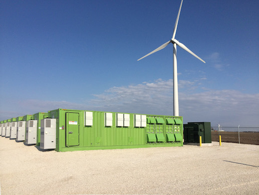
Stern D. I. (2020) How large is the economy-wide rebound effect? Energy Policy 147, 111870. Working Paper Version | Blogpost

Nobel A., S. Lizin, R. Brouwer, S. B. Bruns, D. I. Stern, and R. Malina (2020) Are biodiversity losses valued differently when they are caused by human activities? A meta-analysis of the non-use valuation literature, Environmental Research Letters 15, 070030.

Csereklyei Z. and D. I. Stern (2020) Flying more efficiently: Joint impacts of fuel prices, capital costs and fleet size on airline fleet fuel economy, Ecological Economics 175, 106714. Working Paper Version | Blogpost | Data and Code

Bruns S. B., Z. Csereklyei, and D. I. Stern (2020) A multicointegration model of global climate change, Journal of Econometrics 214(1), 175-197. Working Paper Version | Blogpost | Data

We posted four working papers. Two of those were already published this year and the links are above. The third is a revised version of our paper on the industrial revolution:

Directed technical change and the British Industrial Revolution. December 2020. With Jack Pezzey and Yingying Lu. Blogpost 1, Blogpost 2

The fourth is a nineteen author review for Annual Review of Environment and Resources:

Energy efficiency: What has it delivered in the last 40 years? December 2020. With Harry Saunders et al. Blogpost

We have five papers under review at the moment (three are resubmissions), one revise and resubmit we are working on, and eight more that we are actively working on or trying to finish.

Google Scholar citations exceeded 19,000 with an h-index of 53. I wrote a few more blogposts this year. This is the 10th this year compared to only three last year. Twitter followers rose from 1250 to 1500 over the year. At one point, I actually unfollowed everyone and then added back people I wanted to follow. This made my Twitter feed more manageable and I lost very few followers in the process. 

 

In July, I moved all my email (more than 160k messages) from Outlook on local hard drives to GMail. I use Thunderbird as the front end. Now all my data is in the cloud (everything else is on Dropbox) and can be accessed from anywhere. I still use locally stored applications, so if I want to use specialized software – for example, my econometrics package RATS – I still need to use my own computer.

 

I did 7 external assessments of people for promotion, tenure, or fellowships for universities in Pakistan, Australia, South Africa, USA, Sudan, and Singapore. I'd only done 9 of these previously in my career according to my records. Hard to explain this sudden rush! As a result, I only did 12 reviews for journals, which was lower than typical in the past. And a bunch of papers for EAERE, a proposal for the ARC...

I taught environmental economics and the masters research essay course again. This was the third time I taught the environmental economics course. After a few weeks we had to shift both courses online as I mentioned above. One of the challenges was carrying out a final exam remotely, which I discussed in a workshop ANU ran in the following semester. 

 

Xueting Zhang started as my PhD student.  In the first year, she has been focused on coursework, we are now transitioning to research. I have one other student for whom I am the primary supervisor, Debasish Das. He's working on prepaid metering in Bangladesh and other energy related topics. This involves struggling with a big data set. We only used a small sample in the Energy Insight linked above.

Looking forward to 2021, a couple of things can be predicted:

• I was awarded a Francqui Chair at the University of Hasselt in Belgium for the 2020-21 academic year. So, now I have to come up with ten hours of lectures. What can't be predicted is if I will actually travel to Belgium.
• I'll be teaching environmental economics and the master's research essay course again in the first semester. This year, we are also introducing a year long "Master's Research Project" in parallel with the one semester "essay".
• I'm hoping we get the resubmitted papers and the revise and resubmit published, but that is in the hands of the editors, referees, and journal publishers...
  

Energy Efficiency: What Has It Delivered in the Last 40 Years?

I'm one of nineteen authors of a new review of energy efficiency economics. It was commissioned for the Annual Review of Environment and Resources, where it is still in (second-round) review. The team was put together and led by Harry Saunders and Joyashree Roy.

Over the past four decades different disciplinary approaches independently adopted different definitions of energy efficiency to answer specific problems. Even within economics there are at least three different ideas of energy efficiency. Technical efficiency in economics compares the quantity of inputs used to produce given outputs (or vice versa) to the best practice or frontier level. This is a relative measure of energy efficiency. But economists often talk about energy efficiency in absolute terms too,  measured as either simply an increase in energy services per unit input or using the concept of energy augmenting technological change where the amounts of other inputs and the technology associated with them are held constant. Energy augmenting technological change is usually used when modeling economy-wide rebound, whereas the energy services per unit input might be used when investigating the energy efficiency gap.

The energy intensity of economies (a metric measuring energy consumption per unit of GDP), which is often interpreted as a proxy for energy efficiency, has trended downwards (increasing efficiency) globally and in many major economies over the last century. But as panel (a) below shows, in many regions of the world, especially poorer or hotter regions, energy intensity instead increased. Today, energy intensity is more similar around the world than in the past.

Innovation in energy-saving technologies is an important driver in improving aggregate energy efficiency deployment by lowering costs and inducing adoption. The productivity of numerous energy-using products has improved dramatically. (e.g., lighting had a 10,000-fold improvement in lumens/Watt since the start of the industrial revolution). 

Energy efficiency improvements, in themselves, generally increase economic welfare. But when we consider negative externalities, such as pollution emissions, welfare effects are more ambiguous. Interventions such as improperly calibrated subsidies to improve energy efficiency or mandates to use costly technologies can lead to a reduction in household welfare.

There is still uncertainty and difficulty in measuring economy-wide rebound effects. Rebound may limit the ability to reduce or constrain overall energy use. In general, it makes more sense to address the environmental impacts of energy use with specific environmental policies rather than trying to reduce energy use with energy efficiency policies.

The contribution of different factors to the persistent “energy efficiency gap”, i.e., the difference between the energy consumption observed and the potential energy consumption levels that would result from the adoption of cost-efficient energy efficient technologies and strategies, is still not well understood. Market and regulatory failures, departure of consumer behavior from rational choice theory, lack of information, the principal-agent problem, among other issues may all contribute to the energy efficiency gap.

Policy interventions aimed at overcoming or reducing barriers to energy efficiency deployment target behavioral anomalies and perceived market failures. They include provision of feedback to energy users, the use of social norms, commitment devices, rewards and regulatory mechanisms such as taxes, subsidies, building codes, etc. The literature and evidence are mixed on the effectiveness of each of these, but all seem to show promise to some degree. 

Methodological advances for examining energy efficiency effects on energy use have been substantial. Primary advances include randomized control trials coupled with appropriate econometric methods, developments in econometric methods and lab/field experiments, agent-based modeling formulations, general equilibrium methods, and behavioral science. 

The following diagram summarizes the state of knowledge across different scales and the needed scope of future research:

Future research should bring together researchers from different fields to shed new light onto energy efficiency questions. Examples of such endeavors include: (i) at the micro-level, a better understanding of consumer choice and behavior by combining insights from engineering and the advanced metering and sensing infrastructure, with those from micro-economic theory as well as the theory of choice and with behavioral economists’ models; (ii) at the program evaluation level, there is a need to continue to develop methods to understand causal inferences using econometrics as well as machine learning to better understand program outcomes; (iii) at the macro-level, developing flexible and credible general equilibrium models that also capture environmental and climate externalities outcomes, and that have good input data to enable us to understand the dynamics of energy efficiency improvements across the economy, the environment, and society, are needed.

Francqui Chair

I am one of the two recipients (one is Belgian and one international) of a Francqui Chair at Hasselt University. This sounds like an academic position but actually is a one year appointment during which the chair is supposed to give 10 hours of lectures in their field. I'm not sure yet what they are exactly looking for. But here are Siem Jan Koopman's planned lectures at the University of Antwerpen.

 

So, I'm thinking if I weave my research into a more pedagogical narrative I would be on the right track. I am hoping the lectures will be recorded and I will be able to post them here on Stochastic Trend. My coathors Stephan Bruns and Robert Malina nominated me for this award.

I am hoping I will actually be able to visit Belgium next year assuming that I will be able to access a COVID-19 vaccine.

Asymmetric Carbon Emissions-Output Elasticities

This semester my masters' research essay student, Kate Martin, revisited the topic of whether the carbon emissions-output elasticity is greater in recessions than in economic expansions. In other words, does a 1% increase in output increase carbon emissions by less than a 1% fall in output reduces them?

Sheldon (2017) used quarterly US GDP data and carbon emissions data from the 1950s to 2011 and found that the elasticity in recessions was much larger than in expansions when it was not significantly different to zero. There was also a strong positive drift in emissions of 5.8% p.a.

To measure output, Kate used monthly US industrial production data from 1973 to 2020 and monthly GDP data from 1992 that are available from Macroeconomic Advisers. The advantage of the longer time series is that it covers more recessions and expansions. She also compared this monthly data to quarterly data to test the effect of data frequency. She found that using industrial production and, in particular industrial CO2 emissions rather than total CO2 emissions from fossil fuels, the elasticity is actually larger in expansions but it is not statistically significantly different from the elasticity in recessions. Using GDP data at both monthly and quarterly frequencies and including the last decade of data confirmed Sheldon's basic result.

When Kate restricted the estimation period to the end of 2019, the resulting model projected emissions during the COVID recession (using the reported industrial production data) very well:

This difference between the effect of industrial production and overall GDP on emissions doesn't seem to have been commented on before. However, Eng and Wong (2017) used monthly industrial production data and found that in the short-run the elasticity is symmetric but in the long run the recession elasticity is larger.

Prepaid Metering and Electricity Consumption in Developing Countries

I've written an Energy Insight policy brief for the EEG Programme with my PhD student Debasish Das on prepaid metering and its effect on electricity consumption.

The bottom line is that consumers who are switched to prepaid metering significantly reduce their electricity consumption. 

Debasish is working on a study of the effect of prepaid metering in Bangladesh and some preliminary results are in this paper. This graph shows the estimated difference in monthly electricity consumption between consumers in two areas of Dhaka, Bangladesh around the time that one group was switched to prepaid metering:

 

 

Electricity consumption in the treated group fell by 17%. This graph didn't make it into the final version of the paper, because it was deemed to be too mathy. Debasish has a very large dataset that he obtained from the Bangladesh electric utilities. He's still working on getting this into a usable form. But hopefully we will have some more results soon.

Assessing Students during the Pandemic

Last week I was a panelist at an ANU webinar on assessing students during the current pandemic conditions.

You can watch just my part where I talk about reorganizing my course to deal with online exams:

Or the whole discussion here:

Climate Econometrics and the Carbon Budget

Though I recently abandoned a follow up paper on our Journal of Econometrics climate modeling paper, we are now working on a different one. I'm scheduled to give a presentation (remotely) on it at the American Geophysical Union conference in December. In the course of our research, I ran some simple simulations on our Journal of Econometrics model. This model is a two equation vector autoregression of global surface temperature and radiative forcing with energy balance restrictions imposed. This is done using the concept of multicointegration. But it is still a simple time series model once the complicated estimation is complete.

I ran three scenarios that all have the same peak level of radiative forcing equivalent to doubling CO2:

Single Shock: Forcing is doubled in one year and then the system is allowed to move to equilibrium.

Shock and Maintain: Forcing is doubled suddenly and then that level of forcing is maintained forever. This is the scenario in our published paper and is used to estimate the equilibrium climate sensitivity in general circulation models.

Transient: Forcing is increased linearly for 70 years until the CO2 equivalent would be doubled. Then emissions are cut to zero.

This is what happens to temperature in the three scenarios:

Under the Shock and Maintain scenario, we reach the equilibrium climate sensitivity of 2.78ºC. Under the Transient scenario, the temperature increases by 1.85ºC when emissions are cut to zero and then continues to increase by about 0.3ºC before flatlining. Under the Single Shock scenario, temperature increases quite rapidly, reaching equilibrium in around 40 years with only a 0.98ºC increase.

This is what happens to radiative forcing in the three scenarios:

Under the Single Shock scenario there is a steep fall in forcing after the single pulse of greenhouse gases. A new equilibrium concentration and temperature is reached. Under the Transient scenario the equilibrium level of forcing is much higher even though in both cases emissions are cut to zero. Of course, much more carbon would need to be pumped into the atmosphere to achieve the Transient path as all the time carbon is also being absorbed. This shows the importance of the carbon budget. The total amount of emissions, not just the peak concentration matters. It is interesting that our very simple model seems to pick this up from the data without imposing any information about the carbon budget on the model.

Abandoning a Paper

Now and then it's time to give up on a project. In September 2018, I attended a climate econometrics conference at Frascati near Rome. For my presentation, I did some research on the performance of different econometric estimators of the equilibrium climate sensitivity (ECS) including the multicointegrating vector autoregression (MVAR) that we used in our paper in the Journal of Econometrics. The paper included estimates using historical time series observations (from 1850 to 2014), a Monte Carlo analysis, estimates using output of 16 Global Circulation Models (GCMs), and a meta-analysis of the GCM results.

The historical results, which are mostly also in the Journal of Econometrics paper, appear to show that taking energy balance into account increases the estimated climate sensitivity. By energy balance, we mean that if there is disequilibrium between radiative forcing and surface temperature the ocean must be heating or cooling. Surface temperature is in equilibrium with ocean heat, and in fact follows ocean heat much more closely than it follows radiative forcing. Not taking this into account results in omitted variables bias. Multicointegrating estimators model this flow and stock equilibirum. The residuals from a cointegrating relationship between the temperature and radiative forcing flows are accumulated into a heat stock, which in turn cointegrates with surface temperature. If we have actual observations on ocean heat content or radiative imbalances we can use them. But available time series are much shorter than those for surface temperature or radiative forcing. The results also suggested that using a longer time series increases the estimated climate sensitivity.

The Monte Carlo analysis was supposed to investigate these hypotheses more formally. I used the estimated MVAR as the model of the climate system and simulated the radiative forcing series as a random walk. I made 2000 different random walks and estimated the climate sensitivity with each of the estimators. This showed that, not surprisingly, the MVAR was an unbiased estimator. The other estimators were biased using a random walk of just 165 periods. But when I used a 1000 year series all estimators were unbiased. In other words, they were all consistent estimators of the ECS. This makes sense, because in the end equilibrium is reached between forcing and surface temperature. But it takes a long time.

Each of the GCMs I used has an estimated ECS ("reported ECS") from an experiment where carbon dioxide is suddenly increased fourfold. I was using data from a historical simulation of each GCM, which uses the estimated historical forcings over the period 1850 to 2014. A major problem in this analysis is that the modelling teams do not report the forcing that they used. This is because the global forcing that results from applying aerosols etc depends on the model and the simulation run. So, I used the same forcing series that we used to estimate our historical models. This isn't unprecedented, Marvel et al. (2018) do the same.

In general, the estimated ECS were biased down relative to the reported ECS for the GCMs, but again, the estimators that took energy balance into account seemed to do better. In an meta-analysis of the results, I compared how much the reported radiative imbalance (=ocean heat uptake roughly) from each GCM increased to how much the energy balance equation said it should increase using the reported temperature series, reported ECS, and my radiative forcing series. A regression analysis showed, that where the two matched, the estimators that took energy balance into account were unbiased, while those that did not match, under-estimated the ECS.

These results seemed pretty nice and I submitted the paper for publication. Earlier this year, I got a revise and resubmit. But when I finally got around to working on the paper post-lockdown and post-teaching things began to fall apart.

First, I came across the Forster method of estimating the radiative forcing in GCMs. This uses the energy balance equation:

where F is radiative forcing, T is surface temperature, and N is radiative imbalance. Lambda is the feedback parameter. ECS is inversely proportional to it. The deltas indicate the change since some baseline period. Then, if we know N and T, both of which are provided in GCM results, we can find F! So, I used this to get the forcing specific to each GCM. The results actually looked nicer than in the originally submitted paper. These are the results for the MVAR for 15 CMIP5 GCMs:

The rising line is a 45 degree line, which marks equality between reported and estimated ECSs. The multicointegrating estimators were still better than the other estimators. But there wasn't any systematic variation in the degree of underestimation that would allow us to use a meta-analysis to derive an adjusted estimate of the ECS.

This is still OK. But then I read and re-read more research on under-estimation of the ECS from historical observations. The recent consensus is that estimates from recent historical data will inevitably under-estimate the ECS because feedbacks change from the early stages after an increase in forcing to the latter stages as a new equilibrium is reached. The effective climate sensitivity is lower at first and greater later.

OK, even if we have to give up on estimating the long-run ECS, my estimates are estimates of the historical sensitivity. Aren't they? The problem is that I used the long-run ECS to derive the forcing from the energy balance equation. So, the forcing I derived is wrong. It is too low. I could go back to using the forcing I used previously, I guess. But now I don't believe the meta-analysis of that data is meaningful. So, I have a bunch of estimates using the wrong forcing with no way to further analyse them.

I also revisited the Monte Carlo analysis. By the way I had an on-and-off again coauthor through this research. He helped me a lot with understanding how to analyse the data. But he didn't like my overly bullish conclusions on the submitted paper and so withdrew his name from it. But he was maybe going to get back on the revised submission. He thought that the existing analysis which used an MVAR to produce the simulated data was maybe biased unfairly in favour of the MVAR. So, I came up with a new data-generating process. Instead of starting with a forcing series I would start with the heat content series. From that I would derive temperature, which needs to be in equilibrium with heat content and then using the energy balance equation derive the forcing. To model the heat content I fitted a unit root autoregressive model (stochastic trend) to the heat content reported from the Community GCM with the addition of a volcanic forcing explanatory variable. The stochastic trend represents anthropogenic forcing. The Community GCM is one of the 15 GCMs I was using and it has temperature and heat content series that look a lot like the observations. I then fitted a stationary autoregressive model for temperature with the addition of the heat content as an explanatory variable. The simulated model used normally distributed shocks with the same variance as these fitted models and volcanic shocks.

As an aside, the volcanic shocks were produced by the model:

where rangamma(0.05) are random numbers drawn from a standard gamma distribution with shape parameter 0.05. This is supposed to produce the stratospheric sulfur radiative forcing, which decays over a few years following an eruption. Here is an example realisation:

The dotted line is historical volcanic forcing and the solid line a simulated forcing. My coauthor said it looked "awesome".

So, again, I produced two sets of 2000 datasets. One with a sample size of 165 and one with a sample size of 1000. Now, even in the smaller sample, all four estimators I was testing produced essentially identical and unbiased results! I ran this yesterday. So, our Monte Carlo result disappears. I can't see anything unreasonable about this data generating process, which produces completely different results to the one in the submitted paper. So, I don't see anything to justify one over the other. So, this was the point where I gave up on this project.

My coauthor, who is based in Europe, is on vacation. Maybe he'll see a way to save it when he comes back, but I am sceptical.

How Large is the Economy-Wide Rebound Effect?

Last year, I published a blogpost about our research on the economy-wide rebound effect. The post covers the basics of what the rebound effect is and presents our results. We found that energy efficiency improvements do not save energy. In other words, the rebound effect is 100%. This doesn't mean that improving energy efficiency is a bad thing. It's a good thing, because consumers get more energy services as a result. But it probably doesn't help the environment very much.

I now have a new CAMA working paper, which surveys the literature on this question. Contributions to the literature are broadly theoretical or quantitative. Theory provides some guidance on the factors affecting rebound but does not impose much constraint on the range of possible responses. There aren't very many econometric studies. Most quantitative studies are either calculations using previously estimated parameters and variables or simulations.

Theory shows that the more substitutable other inputs are for energy in production the greater the rebound effect. This means that demand for energy services by producers is more elastic and so reducing the unit costs of energy services increases the amount used by more.

The most comprehensive theoretical examination of the question is Derek Lemoine's new paper in the European Economic Review: "General Equilibrium Rebound from Energy Efficiency Innovation." Lemoine provides the first mathematically consistent analysis of general equilibrium rebound, where all prices across the economy can adjust to a change in energy efficiency in a specific production sector. He shows that the elasticity of substitution in consumption plays the same role as the elasticity of substitution in production: the greater the elasticity, the greater the rebound, ceteris paribus.

Beyond that, the predictions of the model depend on parameter values. The most likely case, assuming a weak response labor to changes in the wage rate, is that the general equilibrium effects increase energy use relative to the partial equilibrium direct rebound effect for energy intensive sectors and reduce it for labor intensive sectors.

Lemoine uses his framework and previously estimated elasticities and other parameters to compute the rebound to an economy-wide energy efficiency improvement in the US. The result is 38%. There are two main reasons why the real rebound might be higher than this. First, most of the elasticities of substitution in production that he uses are quite low because of how they were estimated. Second, an energy efficiency improvement in any sector apart from the energy supply sector does not trigger a fall in the price of energy. A fall in the price of energy would boost rebound. This is because there are no fixed inputs and there are constant returns to scale in energy production.

There are similar issues with simulations from computable general equilibrium models (CGE). The assumptions that modellers make and the parameter values they choose make a huge difference to the results. Depending on these choices, any result from super-conservation, where more energy is saved than the energy efficiency improvement alone would save, to backfire, where energy use increases, is possible.

Rausch and Schwerin estimate the rebound using a small general equilibrium model calibrated to US data. This is somewhere between the typical CGE model and econometric models. They use the putty-clay approach to measuring and modeling energy efficiency. Increases in the price of energy relative to capital are 100% translated into improvements in the energy efficiency of new capital equipment. Once capital is installed, energy and capital must be used in fixed proportions. Rebound in this model depends on why the relative price changes. If the price of energy rises, energy use falls. However, if the price of capital falls energy use increases. These are very strong assumptions, which determine how the data are interpreted. Are they realistic? Rausch and Schwerin find that historically rebound has been around 100% in the US.

Historical evidence also hints that the economy-wide rebound effect could be near 100%. Energy intensity in developing countries today isn't lower than it was in the developed countries when they were at the same level of income. This is despite huge gains in energy efficiency in all kinds of technologies from lighting to car engines. This makes sense if consumers have shifted to more energy intensive consumption goods and services over time. Commuters and tourists on trains in the 19th and early 20th centuries have been replaced by commuters and tourists in cars and on planes in the late 20th and early 21st centuries.

I only found three fully empirical econometric analyses. One of them is our own paper. The others are by Adetutu et al. (2016) and Orea et al. (2015). Both use stochastic production frontiers to estimate energy efficiency. This is a potentially promising approach. Adetutu et al. then model the effect of this energy efficiency one energy use, using an autoregressive model. This includes the lagged value of energy use as an explanatory variable, which means that the long-run effect of all variables is greater in absolute value than the short-run effect. As in the short run, energy efficiency reduces energy use, in the long run it reduces it even more. The result is super-conservation even though short-run rebound is 90%. In Orea et al.'s model, the purely stochastic inefficiency term is multiplied by [1-R(γ'z)] where z is a vector of variables including GDP per capita, the price of energy, and average household size. R(γ'z) is then supposed to be an estimate of the rebound effect. But really this is just a reformulation of the inefficiency term – nothing specifically identifies R(γ'z) as the rebound effect.

In conclusion, the economy-wide rebound effect might be near 100%. But I wouldn't describe the evidence as conclusive. Both our research and the historical investigations might be missing some important factor that has moved energy use in a way that makes us think it is due to changes in energy efficiency, and Rausch and Schwerin make very strong assumptions about analysing the data.

Designing Future Electricity Markets: Evolution Rather than Revolution

We have a new working paper on designing wholesale electricity markets with high levels of zero marginal cost intermittent energy sources. The paper reports on the findings of a session on this topic at the Future of Electricity Markets Summit that was held in November last year in Sydney. Gordon Leslie led the writing with contributions from myself, Akshay Shanker, and Mike Hogan. The session itself featured papers by Paul Simshauser, Mike Hogan, Chandra Krishnamurthy (a paper coauthored with Akshay and myself), and Simon Wilkie.

Imagine the future where fossil fuel generation has disappeared and generation consists of intermittent sources like solar and wind. The cost of producing more electricity with these technologies is essentially zero – the marginal cost of production is zero – once we have invested in the solar panels or wind turbines. But that investment is costly. How would markets for electricity work in this situation? The naive view is that introductory economics tells us that the price in competitive markets, like many wholesale electricity markets (e.g. Australia's National Electricity Market – the "NEM"), is equal to marginal cost. If renewables have zero marginal cost, then the price would be zero. So, an "energy only market" where generators are paid for the electricity they provide to the grid won't be viable and we need a total redesign.

But the consensus in our session was that zero marginal cost generation doesn't mean that energy only markets can't work. Marginal cost of production isn't as important as marginal opportunity cost. Hydropower plants have a near zero marginal cost of production but if they release water when the price of electricity is low, they forego generating electricity when the price is high. Releasing water has an opportunity cost. Mike Hogan pointed out that the same is true of reserves more generally. There will also be electricity storage including pumped hydropower as well as batteries and other technologies in the future. The Krishnamurthy paper focused in particular on the role of storage. The price these receive should also be determined by opportunity cost. Even without storage and reserves there should be a market equilibrium with a non-zero price as long as there is sufficient flexibility of demand for electricity:

Intermittent renewables supply to the market however much power, Rt, that they can generate. They can't supply unlimited power at zero marginal cost... The market clearing price is p, where the demand curve, Dt, crosses the vertical supply curve. Price does not equal marginal cost of production. Of course, the quantity and price is continually fluctuating. But, if, on average, the revenues are insufficient to cover the costs of investment, generation capacity will shut down and exit the market until long-run equilibrium is restored. Storage has the effect of making the supply curve more elastic like the St supply curve in this graph:

In this example, storage lowers the price and increases the quantity of electricity consumed. This is when storage is discharging electricity. When it is charging, it will raise the price relative to the case with no storage. Storage has the effect of reducing volatility.

This is of course very simplified. The real world is more complicated. The paper shows that increasing intermittent generator penetration increases the importance of adequately pricing scarcity and all network constraints and services. Wind generation tends to colocate in the best wind resource areas overloading the gird. Locational marginal pricing pricing is required to deliver investment incentives for the right technologies to locate at the right locations to efficiently maintain a stable and reliable electrical network as discussed by Katzen and Leslie (2020). The NEM currently only has a spot market that schedules generation for each 5 minute interval. A day-ahead market could help in valuing the provision of flexible generation and storage. The current charges for transmission costs in the NEM also disincentivize grid-scale storage. Electricity users pay for these costs. This makes sense when the user is an end-user. But storage is treated as a customer and also pays these charges.  So "fresh electricity" where only one set of charges is paid has a cost advantage over stored electricity.

In conclusion, electricity markets need to evolve to provide the correct incentives to generation and storage. A total rethink isn't needed.