The Impact of Electricity on Economic Development: A Macroeconomic Perspective

I have a new working paper out, coauthored with Paul Burke and Stephan Bruns. The paper is one of those commissioned for the first year of the Energy for Economic Growth program, which is funded by the UK Department for International Development and directed by Catherine Wolfram.  The paper was actually completed in January 2017, but there has been a lot of delay in getting approval for publication. The project and the paper focuses on the role of electricity in economic development in Africa and South Asia, the two regions of the world where electricity is least accessible.

Access to and consumption of electricity varies dramatically around the world. Access is lowest in South Sudan at 4.5% of households, while consumption ranges from 39 kWh per capita – this includes all uses of electricity not just household use – in Haiti to 53,000 kWh per capita in Iceland – driven by aluminum smelting. Consumption is 13,000 kWh per capita in the US. Electricity use and access are strongly correlated with economic development, as theory would suggest:

Access and consumption have increased strongly in many poorer countries in recent years – will this have beneficial effects on development? The specific questions that DFID asked us to answer were:

• How serious do electricity supply problems have to be in order to constitute a serious brake on economic growth?

• To what degree has electrification prolonged or accelerated economic growth?

• What can be learned from the development experience of countries that have invested successfully in electrification?

In principle, it should be easier to find evidence for causal effects using more disaggregated micro level data as some variables can more easily be considered exogenous, and randomized trials and other field experiments are possible. On the other hand, growth is an economy-wide, dynamic, and long-term process with effects that cannot usually be captured in micro studies. Therefore, macroeconomic analysis is also needed. Our paper is complemented by a paper covering the microeconomic aspects of these questions.

Despite large empirical literatures – such as that on testing for Granger casuality between electricity use and economic growth – and suggestive case evidence, we found few methodologically strong studies that establish causal effects for electricity use, access, infrastructure, or reliability on an economy-wide basis. The best such study that we found is a paper by Calderon et al. in the Journal of Applied Econometrics. But this paper actually tests the effects of an aggregate of different types of infrastructure on growth.

We propose that future research focuses on identifying the causal effects of electricity reliability, infrastructure, and access on economic growth; testing the replicability of the literature; and deepening our theoretical understanding of how lack of availability of electricity can be a constraint to growth.

Annual Review 2017

I've been doing these annual reviews since 2011. They're mainly an exercise for me to see what I accomplished and what I didn't in the previous year. As I mentioned in last year's review, I am still struggling with work-life balance. It feels like that there is never enough time to get the work done I need to do and I am always making excuses for not getting things done. So, stopping and looking at what I did get done can help provide some perspective.

I was IDEC (Crawford's economics program) director till the end of the year. Ligang Song will take over as IDEC director in 2018. We continued to work on developing and seeking approval for new programs. We made some progress, but the final outcome will only be known in 2018 (hopefully). There was also quite a lot of work on the review of the Crawford School, the future of Asia-Pacific economics at ANU, economics at Crawford and ANU etc. The Arndt-Corden Department of Economics is officially a separate organizational unit from IDEC. Our plan is that going forward Arndt-Corden will represent the research, outreach, and PhD program components of all the economics activity at Crawford and IDEC will continue as the masters teaching program. This too is a work in progress. 

ANU environment and resource economists, Paul Burke, Frank Jotzo, Quentin Grafton, Jack Pezzey, and me

I made two international trips - one to Singapore and one to Europe and two short trips in Australia to Brisbane and Melbourne.  I went to the Singapore meeting for the IAEE international conference. My wife, Shuang, and son, Noah, came along too and we extended our stay to spend time in Singapore. We took the new direct flight from Canberra to Singapore, which is very convenient. From February there will also be Qatar Airways flights from Canberra, but apparently they will stop in Sydney before continuing to Singapore. That will just save time (maybe) on going between terminals in Sydney. To get to Europe I flew to Adelaide and then took Emirates via Dubai.

I was in Brisbane for the AARES conference. I have always found that the conference is much more dominated by agricultural economics than the journal but almost everything at the conference this time was agriculture related. Most of the environment papers dealt with agricultural impacts. I decided not to go in 2018, though the program is looking more balanced.

In December I traveled to Spain, Germany, and Israel. I gave a seminar at ICTA at the Autonomous University of Barcelona on the role of energy in modern economic growth. This was part of a series of seminars funded by the Maria de Maeztu program.

Speaking at ICTA, UAB, Barcelona

From there, I went on to Germany to work with Stephan Bruns on our ARC project and climate change paper. Alessio Moneta also visited from Pisa for a couple of days. Totally by coincidence, I arrived in Göttingen on the same day as Paul Burke who was touring Germany as part of his Energy Transition Hub activities:

Stephan Bruns, Krisztina Kis-Katos, Paul Burke, and me in Göttingen

We made quite good progress on both projects while I was there, but there is still much to do. We are just over the halfway point with the ARC DP16 project. One short paper is already published in Climatic Change, which discusses the accuracy of projections of future energy intensity. We also have another working paper on the restructuring of the US electricity generation industry and energy efficiency and have a paper under review on aircraft fuel economy.

We also completed and submitted our paper on the macroeconomic aspects of electricity and economic development for the DFID funded EEG project. Publication of the working papers and announcement of the next stages of the project have been much delayed, but there should be news on the latter soon. Together with our PhD student Akshay Shanker, I made a lot of progress on our contribution to a Handelsbanken Foundation funded project headed by Astrid Kander. Well, Akshay did most of the work... The paper  – about why energy intensity declines over time – will now be part of Akshay's PhD thesis.

I published fewer papers than last year, which isn't a surprise, as last year was a record year. There were five articles with a 2017 date:

Stern D. I., R. Gerlagh, and P. J. Burke (2017) Modeling the emissions-income relationship using long-run growth rates, Environment and Development Economics 22(6), 699-724. Working Paper Version | Blogpost

Stern D. I. (2017) How accurate are energy intensity projections? Climatic Change 143, 537-545. Working Paper Version | Blogpost

Zhang W., D. I. Stern, X. Liu, W. Cai, and C. Wang (2017) An analysis of the costs of energy saving and CO2 mitigation in rural households in China, Journal of Cleaner Production 165, 734-745. Working Paper Version | Blogpost
 
Stern D. I. and J. van Dijk (2017) Economic growth and global particulate pollution concentrations, Climatic Change 142, 391-406. Working Paper Version | Blogpost

Stern D. I. (2017) The environmental Kuznets curve after 25 years, Journal of Bioeconomics 19, 7-28. Working Paper Version | Blogpost

and there is one in press at the moment:

Bruns S. B. and D. I. Stern (in press) Overfitting bias and p-hacking in Granger-causality testing: Meta-evidence from the energy-growth literature, Empirical Economics. Working Paper Version | Blogpost

I also published a comment on a paper in Scientometrics:

Stern D. I. (2017) Comment on Bornmann (2017): Confidence intervals for journal impact factors, Scientometrics 113(3), 1811-1813. Blogpost

Follow the links to the blogposts to find out more about each paper.

I also published between 1 and 3 book chapters. It's often hard to work out when exactly a book chapter is published or not! This one is definitely published and it's open access for now. I only do book chapters where I can update an existing survey paper for the purpose. I posted 5 working papers, two of which have already been published and two are in the review process. In total, 6 papers are currently submitted, resubmitted, or in revision for resubmission.

Citations almost reached 14,000 on Google Scholar (h-index: 45) and will be well in excess of that for the end of 2017 when all this year's citations are finally included in Google's database.

I became an editor at PeerJ as part of their expansion into the environmental sciences. So far, I haven't actually handled a paper but I'm sure there will be some relevant submissions soon.

On the teaching side, I convened Masters Research Essay for the first time in the 1st Semester and taught Energy Economics for the last time for now in the second semester. My first PhD student here at Crawford, Alrick Campbell, received his PhD at the July graduation ceremony. He is currently a lecturer at the University of the West Indies in Jamaica.

I have been blogging even less this year than last. This will be the 19th post for 2017, whereas last year there were 35. Lack of time and increased use of Twitter are to blame. My Twitter followers now number more than 750, up from over 500 last year. The most popular blogpost this year was "Confidence Intervals for Journal Impact Factors".

Looking forward to 2018, it is easy to predict a couple of things that will happen that are already organized:

1. As mentioned above, I am ending my term as director of our economics program, IDEC, at the end of this calendar year. I am hoping to be able to focus a bit more on my research and get more balance in the coming year.

2. I will be the convener for Masters Research Essay and teach Environmental Economics in the first semester. I last taught environmental economics 10 years ago at RPI, so it will be quite a lot of work. I was getting a bit tired of teaching Energy Economics and if I did this course, Paul Burke could teach one of our compulsory first year masters microeconomics courses, so I decided to take it on. Both these courses are in the 1st semester and so I won't be teaching in the 2nd semester.

3. Early in the new year we will put out a working paper for our time series analysis of global climate change. We are currently revising the paper to resubmit to the Journal of Econometrics.

Nothing came of the job I applied for last year beyond the Skype interview, but I applied for another one this year...

Data and Code for "Energy and Economic Growth: The Stylized Facts" and an Erratum

Following a request for our estimation code we have now completed a full replication package for our 2016 Energy Journal paper and uploaded it to Figshare.

While we were putting this together we noticed some minor errors in the tables in the published paper. The reported standard errors of the coefficients of lnY/P in Tables 2 and 3 for the results without outliers are incorrect. We accidentally pasted the standard errors from Table 5 into Tables 2 and 3. The correct versions of Tables 2 and 3 should look like this:

The standard errors for unconditional convergence in Tables 4 and 6 are also incorrect. The reported standard errors are not robust and one was completely wrong. The tables should look like:

None of these errors results in the significance level in terms of 1%, 5% etc. changing.

Distribution of SNIP and SJR

My colleague Matt Dornan asked me about the distribution of the journal impact factors SNIP and SJR. Crawford School has used SNIP to compare journal rankings across disciplines. It is a journal impact factor that is normalized for the differences in citation potential in different fields. This makes it reasonable to compare Nature and the Quarterly Journal of Economics, for example. Nature looks like it has much higher impact using the simple Journal Impact Factor that just counts how many citations articles in a journal get. But taking citation potential into account, these journals look much more similar. SJR is an iterative indicator that takes into account how highly cited the journals which cite the journal of interest are. It is similar to Google's pagerank algorithm. It also can be compared across disciplines. SJR is more an indicator of journal prestige or importance rather than simple popularity. I've advocated SJR as a better measure of journal impact as some journals in my area have high citations but those are not in the really highly cited journals.

I assumed the distribution of these indicators was highly skewed with most journals having low impact. But I also assumed that the log of these indicators might be normally distributed as citations to individual papers is roughly log-normally distributed. It turns out that the log of SNIP is still a bit skewed, but not that far from normal:

On the other hand the log of SJR remains highly non-normal:

There is a small tail of high prestige journals and then a big bulk of low prestige journals and a huge spike at SJR = 0.1. It makes sense that it is harder to be prestigious rather than just popular, but still I am surprised by how extreme the skew is. The distribution appears closer to an exponential distribution than a normal distribution.

Barcelona Talk

I'll be giving a presentation in the "distinguished speakers series" at ICAT, Autonomous University of Barcelona on 5th December. I just wrote the abstract:

The Role of Energy in the Industrial Revolution and Modern Economic Growth

Abstract: Ecological and mainstream economists have debated the importance of energy in economic growth. Ecological economists usually argue that energy plays a central role in growth, while mainstream economists usually downplay the importance of energy. Using the (mainstream) theory of directed technological change, I show how increasing scarcity of biomass could induce coal-using innovation in Britain, resulting in the acceleration in the rate of economic growth known as the Industrial Revolution. Paradoxically, industrialization would be delayed in countries with more abundant biomass resources. However, as energy has become increasingly abundant, the growth effect of additional energy use has declined. Furthermore, both directed technological change theory and empirical evidence show that innovation has increasingly focused on improving the productivity of labor rather than that of energy. This explains the focus of mainstream economic growth models on labor productivity enhancing innovation as the driver of economic growth.

The paper will draw on my 2012 paper with Astrid Kander – it shares the same title after all – my recent working paper with Jack Pezzey and Yingying Lu, and maybe my ongoing work with Akshay Shanker on understanding trends in energy intensity in the 20th and 21st Centuries. The talk is for an interdisciplinary audience, so that will be challenging, but I think I can do it :)

Political Bias in My Teaching?

I've long been curious about what students in my classes think about my political position. So, I finally decided to ask them. I added a bonus question for 1 point on top of the 100 points available for the final exam in my Energy Economics course. The question read:

Bonus question (1 point): 
This question relates to potential political bias in my presentation of the course material. Based on the content of the course, which political party do you think I voted for in the last Federal senate election?

a. Greens
b. Labor
c. Liberal
d. Liberal Democrats
e. Australian Sex Party
f. Christian Democratic Party

Actually, ten parties ran at the last election for the two available senate seats representing the ACT, but I thought it would be better to keep the list a little more manageable.

The distribution of answers was as follows:

Greens: 2
Labor: 5
Liberal: 5
Liberal Democrats: 5
Australian Sex Party: 0
Christian Democrats: 0

Assuming that everyone who picked Liberal Democrats knows what it is - a libertarian party - there is a perceived rightward bias. But there are a lot of foreign students who might assume it is a more centrist party. Or people might have assumed that if I listed a bunch of parties they hadn't heard of, one of those must be the right answer.

What would no bias look like? Maybe something more like Green 2, Labor 7, Liberal 7, Liberal Democrat 1 or 3,7,6,1, which is closer to the voting pattern. Or maybe even further to the left as most academics including economists in Australia probably vote for Labor, so that would be the default assumption unless they perceived a strong bias in my teaching?

What Do Crawford School Economists Do?

I'm doing quite a bit of background work for our School Review, a review of the Future of Asia-Pacific Economics etc. The following table is based on the self-identified "Fields of Research" of core Crawford economics faculty. Most people chose more than one field. If, for example, someone chose three fields, then I attributed 1/3 of an FTE to each for that person. The result looks like this:

Our research foci are economic development and growth, environmental and resource economics, and international economics and finance. The (non-geographical) fields that we rank best in globally in RePEc are: Environment 7, Energy 7, Resources 11, Agriculture 23, Growth 29, International Trade 32, Development 39. So, this focus also is where we perform well.

Most Crawford economists have countries that they focus on. Using a similar approach I put together this table:

Naturally, Australia is number one, then follow China, Japan, Indonesia, and Vietnam. In RePEc, we rank 4th in the SE Asia ranking, 18th in Central/Western Asia (which actually includes South Asia), and 39th in the China subject ranking. This reflects more of our historical focus, while the current faculty is more focused on NE Asia. We don't have any current faculty with a professed interest in Thailand, for example! Of course, there is also less competition in research on SE Asia than on China and so that will also affect our ranking.

Impact Factors for Public Policy Schools

As part of our self-evaluation for the upcoming review of the Crawford School, I have been doing some bibliometric analysis. One thing I have come up with is calculating an impact factor for the School and some comparator institutions. This is easy to do in Scopus. It's the same idea as computing one for an individual or a journal, of course. I am using a 2016, 5 year impact factor. Just get total citations in 2016 to all articles and reviews published in 2011-2015. Divide by the number of articles. Here are the results with 95% confidence intervals:

The main difficulty I had was retrieving articles for some institutions such as the School of Public Affairs at Sciences Po. Very few articles came back for various variants of the name that I tried. I suspect that faculty are using departmental affiliations. I had a similar problem with IPA at LSE. So, I report the whole of LSE in the graph. It is easy to understand this metric in comparison to journal impact factors. As an individual metric the confidence interval will usually be large, though my 2016 impact factor was 5.9 with a 4.2 to 7.5 confidence interval. That's more precise than the estimate for SIPA.

More on Millar et al.

Millar and Allen have an article in the Guardian explaining what their paper really says. They say that existing ESMs assume too little cumulative emissions by the 2020's when atmospheric carbon dioxide will be higher than now and so temperature higher than now. But we have already reached that level of cumulative emissions and so we need to do an adjustment to the graph of cumulative emissions vs temperature. But no change to the graph of temperature vs. current concentration of CO2. The discrepancy arises because of uncertainty in cumulative emissions. Models have backfilled this estimate from other variables. Then they say that human induced warming is 0.93C and so that is the temperature baseline of their shifted frame of reference:

The argument of critics like Gavin Schmidt, Zeke Hausfather, and me that the estimate of current human-induced warming is too low still stands. And this means that the remaining carbon budget is smaller than argued by Millar et al. Any likely path to 1.5 degrees will require exceeding that temperature and then bringing radiative forcing down again.

Is the Carbon Budget for 1.5 Degrees Much Larger than We Thought?

An article in Nature Geoscience by Millar et al. on carbon budgets has attracted a lot of attention and debate.* A blogpost by the lead author explains that current human-induced warming has increased in the 2010's by 0.93C over the the 1861-1880 period, while the mean CMIP5 climate model run projected that given cumulative carbon emissions to date the temperature should be 0.3C warmer than that. They argue that that means that the remaining carbon emissions budget allowed for staying within a 1.5C increase in temperature is larger than previously thought as we have 0.6C to go at this point rather than 0.3C. I think there a number of issues with this claim.

First, the value for human-induced warming is based on averaging the orange line in this graph:

The orange line is derived by fitting estimated radiative forcing to observed temperature given by the HADCRUT4 dataset by regression. HADCRUT4 shows less increase in surface temperature than either the GISS or Berkeley Earth datasets because of how it covers the polar regions, in particular.
Using the Berkeley Earth dataset, the temperature increase from the 1861-80 mean to the 2010's mean – shown by black lines in this graph:

is 1.1C. As you can see, even that increase is assuming that conditions during the "hiatus" are more usual than those during the post-2014 increase in temperature. 0.93C is a very conservative estimate of warming to date. Though the recent period was affected by El Nino conditions, it's possible that it represents catching up to the long term trend rather than an excursion above the trend. Throughout the hiatus period ocean heat content was increasing. I do think it is likely that the jump in temperature in the last two years is a recoupling of surface temperature to this more fundamental trend. We have a paper under review that supports this view.**

Also, I think that averaging the orange trend line in the previous graph definitely is too conservative given the strongly non-stationary behavior of the trend. The most recent estimate of the trend would be a better guess.

Second, I think there are a few reasons*** why we might update the carbon budget (as measured from the beginning of the Industrial Revolution):

1. Our estimate of the transient climate sensitivity changes – we think that the short-run temperature for a given concentration of carbon dioxide in the atmosphere is higher or lower than we previously thought.

2. Our estimate of the airborne fraction changes – our estimate of the amount by which the carbon dioxide in the atmosphere increases in reaction to a given amount of emissions changes. CO2 in the atmosphere has increased by about half cumulative emissions.

3. Our estimate of non-CO2 forcing changes. There are important other sources of radiative forcing such as methane and sources of negative forcing such as sulfate aerosols.

Observations of warming to date, isn't one of these. So the paper is implicitly saying that these observations lead them to reduce their estimate of the climate sensitivity.

Third, though the paper says that Earth System Models overestimated warming to date, it seems that the authors use the same models to estimate the remaining carbon budget.

* I have extensively revised this post following a comment from Myles Allen, one of the paper's authors. Also, I realized that the second part of the post didn't really make much sense, so I deleted it.

** The paper has been in review since February, but we haven't posted a working paper, as one of my coauthors didn't want to do so before receiving referee comments.

*** The emissions path also affects the carbon budget as we can see from the mean values for the various RCP paths in the graph below from Millar et al. and the difference between the red plume of RCP paths and the grey plume which are paths where emissions grow at a constant 1% per annum rate. The slower we release carbon, the bigger the budget.

Confidence Intervals for Journal Impact Factors

Is the Poisson distribution a short-cut to getting standard errors for journal impact factors? The nice thing about the Poisson distribution is that the variance is equal to the mean. The journal impact factor is the mean number of citations received in a given year by articles published in a journal in the previous few years. So if citations followed a Poisson distribution it would be easy to compute a standard error for the impact factor. The only additional information you would need besides the impact factor itself, is the number of articles published in the relevant previous years.

This is the idea behind Darren Greenwood's 2007 paper on credible intervals for journal impact factors. As he takes a Bayesian approach things are a little more complicated in practice. Now, earlier this year Lutz Bornmann published a letter in Scientometrics that also proposes using the Poisson distribution to compute uncertainty bounds - this time, frequentist confidence intervals. Using the data from my 2013 paper in the Journal of Economic Literature, I investigated whether this proposal would work. My comment on Bornmann's letter is now published in Scientometrics.

It is not necessarily a good assumption that citations follow a Poisson process. First, it is well-known that the number of citations received each year by an article, first increases and then decreases (Fok and Franses, 2007; Stern, 2014) and so the simple Poisson assumption cannot be true for individual articles. For example, Fok and Franses argue that for articles that receive at least some citations, the profile of citations over time follows the Bass model. Furthermore, articles in a journal vary in quality and do not all each have the same expected number of citations. Previous research finds that the distribution of citations across a group of articles is related to the log-normal distribution (Stringer et al., 2010; Wang et al., 2013).

Stern (2013) computed the actual observed standard deviation of citations in 2011 at the journal level for all articles published in the previous five years in all 230 journals in the economics subject category of the Journal Citation Reports using the standard formula for the variance

where Vi is the variance of citations received in 2011 for all articles published in journal i between 2006 and 2010 inclusively, Ni is the number of articles published in the journal in that period, Cj is the number of citations received in 2011 by article j published in the relevant period, and Mi is the 5-year impact factor of the journal. Then the standard error of the impact factor is √(Vi/Ni ).

Table 1 in Stern (2013) presents the standard deviation of citations, the estimated 5-year impact factor, the standard error of that impact factor, and a 95% confidence interval for all 230 journals. Also included are the number of articles published in the five year window, the official impact factor published in the Journal Citation Reports and the median citations for each journal.

The following graph plots the variance against the mean for the 229 journals with non-zero impact factors:

There is a strong linear relationship between the logs of the mean and the variance but it is obvious  that the variance is not equal to the mean for this dataset. A simple regression of the log of the variance of citations on the log of the mean yields:

where standard errors are given in parentheses. The R-squared of this regression is 0.92. If citations followed the Poisson distribution, the constant would be zero and the slope would be equal to one. These hypotheses are clearly rejected. Using the Poisson assumption for these journals would result in underestimating the width of the confidence interval for almost all journals, especially those with higher impact factors. In fact, only four journals have variances equal to or smaller than their impact factors. As an example, the standard error of the impact factor estimated by Stern (2013) for the Quarterly Journal of Economics is 0.57. The Poisson approach yields 0.2.

Unfortunately, accurately computing standard errors and confidence intervals for journal impact factors appears to be harder than just referring to the impact factor and number of articles published. But it is not very difficult to download the citations to articles in a target set of journals from the Web of Science or Scopus and compute the confidence intervals from them. I downloaded the data and did the main computations in my 2013 paper in a single day. It would be trivially easy for Clarivate, Elsevier, or other providers to report standard errors.

References

Bornmann, L. (2017) Confidence intervals for Journal Impact Factors, Scientometrics 111:1869–1871.

Fok, D. and P. H. Franses (2007) Modeling the diffusion of scientific publications, Journal of Econometrics 139: 376-390.

Stern, D. I. (2013) Uncertainty measures for economics journal impact factors, Journal of Economic Literature 51(1), 173-189.

Stern, D. I. (2014) High-ranked social science journal articles can be identified from early citation information, PLoS ONE 9(11), e112520.

Stringer, M. J, Sales-Pardo, M., Nunes Amaral, L. A. (2010) Statistical validation of a global model for the distribution of the ultimate number of citations accrued by papers published in a scientific journal, Journal of the American Society for Information Science and Technology 61(7): 1377–1385.

Wang, D., Song C., Barabási A.-L. (2013) Quantifying long-term scientific impact, Science 342: 127–132.

Interview with Western Cycles Blog

Alejandro Puerto is a 20 year old who lives in Cuba. He has written: "Western Cycles: United Kingdom" a book that covers the economic and political history of the UK from 1945 onwards. He maintains a website of the same name that showcases his writing. You can also follow him on Twitter. He asked me whether I would I would do an interview for his blog. Here it is:

When did you became interested in the energy and the environment on economics?

I was interested in the environment from an early age and so I studied geography, biology (and chemistry) in the last 2 years of high school in England (1981-3) and then went on to study geography at university (in Israel). I had to pick another field and initially chose business as something practical but quickly switched to economics. I then realised that economics could explain a lot of geography and environmental trends. It was only when I went to do my PhD starting in 1990 that the faculty at Boston University at the Center for Energy and Environmental Studies which was linked to the Geography Department there were really focused on the role of energy in the economy and environmental trends that I became interested in understanding the role of energy. So I got a PhD in geography officially but had quite a lot of economics training and over time drifted closer to economics, so now I am even director of the economics program at the Crawford School of Public Policy at ANU.

I think that my generation is more informed on climate change because of the work of people like you. Do you think the same? Describe us some of your research.

Well, I think it has just become a much bigger and obvious issue as the global temperature has increased. The awareness of what is happening has been driven by people in the natural sciences. I have done some research applying time series models used in macroeconomics to modelling the climate system and though our first paper was published in Nature in 1997 and we have been cited on that in IPCC reports it has largely been on the fringes of climate science. My view of that research is that it takes an entirely different approach to modelling the system than most climate scientists use (mostly they use big simulation models called GCMs) and finds similar results which strengthens their conclusions. Most of my research has been on the role of energy in economic growth and the effect of economic growth on emissions and concentrations of pollutants. The effect of energy on growth is much more complicated than many people think – it seems that energy is more important as growth driver in the past in the developed world – adding energy when you have little has more effect than when you already have a lot. On pollution I’ve argued that the idea of the environmental Kuznets curve – that as countries get richer eventually growth will actually be good for the environment and reduce pollution is either outright wrong or too simplified. Instead in fast growing countries like China, growth overwhelms efforts to reduce pollution, while in slower growing developed economies clean up can happen faster than growth.

The Paris Summit filled your expectations as an environmental economist?

It was probably better than expected give the lack of success in getting agreement before then. Countries pledges are too little to reach the goal of limiting warming to 2C and we will probably have to remove carbon from the atmosphere in a big way later in this Century. The real question is whether countries will actually fulfil their voluntary pledges. OTOH low-carbon technology is developing fast and that is a positive that is making achieving the goals looking more possible.

How dangerous would be the environmental policy of the United States under the Trump administration on climate change?

It will delay action, unclear how much effect it will really have. Encouraging the development of new technology is important and having the largest and leading economy not focused on that is a negative. The US can’t actually leave till late 2020 and Trump has left the door open to submitting a weaker INDC in the interim and claiming victory. The US will still be involved in UNFCCC talks etc.

What do you think about the emissions of developing countries as they become industrious?

Developing country emissions are now larger than developed country emissions. But there is a big difference between China which now has higher per capita emissions than the European Union and say India which has still very low per capita emissions. China needs to take action and has made a moderately strong pledge. We should expect much less from India say. India is, though, strongly encouraging renewables development. Hopefully, technology is advancing fast enough that the poorest countries will end up going down a lower carbon path anyway as fossil fuel technologies gradually phase out.

Since 2006 China has become the greatest global polluter and emissions still growing continuously. China has no plans for decrease these emissions until 2030. What do you think about the attitude of this country?

They say they will peak emissions by 2030. In terms of reduction in emissions intensity per dollar of GDP their goal is quite strong. In the last 3 years Chinese CO2 emissions have been constant. Some argue they are already peaking now. I am a bit more skeptical. We need to see a few more years. There are several reasons why China is pursuing a fairly strong climate policy including energy security, encouraging innovation and reducing local air pollution as well as realising that they can benefit a lot from reducing their own emissions because they are such a large part of the problem.

In the long term, which kind of renewable energy would be the first to think about? Solar? Wind?

Solar – it has a greater potential total resource and looks like eventually prices will be below wind. Wind of course is strong in places without much sunshine like the Atlantic Ocean off NW Europe. I’m concerned though about the environmental impact of lots of wind power. In the long-run I’m still hoping for fusion to work out :)

Tell us about one of your favorite posts published by you on Stochastic Trend.

I’ve done less blogging recently as I now use Twitter for short things. Most of the posts are excerpts from papers or discussions of new papers. The most popular blogpost this year with visitors is:

http://stochastictrend.blogspot.com.au/2017/03/from-wood-to-coal-directed-technical.html

Where I discuss our working paper on the role of coal in the Industrial Revolution. The research and writing of this paper took a very long time and I was really happy to be able to announce to the world that it was ready.

Do you drive an electric car?

No, I don’t have a driving licence. My wife drives and we have a car but it is a large petrol-engined car that is not very efficient. We don’t drive it much though. We’ve driven less than 30,000 km since buying it in 2007.

Have you ever visited Cuba? Are you interested? There are a lot of 1950s cars, but there are places with tropical nature.

No, I haven’t been to Cuba. The only place I’ve been in Latin America is Tijuana, Mexico. I’m not travelling that much recently as we now have a 1 1/2 year old child. But Cuba probably wouldn’t be high on my agenda. I travel mostly to either visit family or go to academic conferences and work with other researchers. The only time I flew somewhere outside the country I was living in just to go on vacation was when I flew from Ethiopia to Kenya. I was at an IPCC meeting in Ethiopia.

Error in 2014 Energy Journal Paper

I hate looking at my published papers because there are often typos in them which I didn't catch at the proofs stage...This time my coauthor, Stephan Bruns, found one in our 2014 paper in the Energy Journal: "Is There Really Granger Causality Between Energy Use and Output?" In Table 1, which describes the details of the studies in our meta-analysis, the control variable labeled "energy production" should actually be labeled "energy price". Energy production would be a weird control variable...

After digging into our draft files, it turns out I changed "energy pr." to "E Prod." systematically in this table just before we resubmitted it to the journal. I also added a footnote: "E Prod.=Energy Production". I don't know why I did this. I would have thought I would have asked, Christian Gross, who made the original version of the table, before doing this, but I can't find any email to prove that...

Robots, Artificial Intelligence, and the Future of Work

I think that robots/artificial intelligence and the future of work is a hugely important topic. This is a very active research field but it seems to me that people (some informed by this research but most without referring to the research) are rushing to one of two conclusions. The first of these conclusions is that up till now economic growth has resulted in rising wages and full employment and so it surely will in the future too. The other is that robots must mean structural unemployment and so the solution is to introduce universal basic income or some similar redistributive policy.

I don't think either is necessarily true. In the past, the elasticity of substitution between labor and capital seems to have been less than one - both inputs were essential in production. Also, the two inputs are q-complements - an increase in capital per worker results in an increase in the marginal product and, therefore, wage of a worker. But it's possible that now, or in the future, that the elasticity of substitution between labor and capital is or will be greater than unity so that labor is not an essential input. Or that there are techniques that are designed just to use machines. Acemoglu and Restrepo (2016) assume that as some low-skilled tasks become automated other new high-skilled tasks are introduced. But there may be limits to people's cognitive ability. Most people aren't intelligent enough to be engineers and scientists. And the people that are intelligent enough now, might be worse than artificial intelligences in the future.

The other premature conclusion is that, definitely things are different now, and robots will result in structural unemployment or immiserizing growth, so that government intervention is needed. Usually, universal basic income is mentioned. Sachs et al. (2015) argue immiserizing growth is possible. This is one of the better papers out there I think, but still the framework is quite limited. as technological change is exogenous. It is possible that there is some self-correcting mechanism similar to that in Acemoglu's (2003) paper on capital- and labor-augmenting technical change. In that model, capital-augmenting technical change is possible for a while, but it introduces forces that return the economy to a pure labor-augmenting technical change path. Another important question is whether people have a preference to have at least some of the goods and services they consume produced by humans. Sachs et al. assume that utility is a Cobb-Douglas function of automatable and non-automatable goods. That means that consumption of human made goods could become infinitesimally small in theory.

I think we need to consider a range of models as well as empirical evidence before we can say what kind of policy, if any, is needed.

I wanted to do research on this and started doing some research on this but concluded that it is not realistic given my limited time for research because of my administrative - I am still director of our International and Development Economics Program - and parenting roles and my existing research commitments. Twitter isn't the only reason that I haven't updated this blog in 2 1/2 months. Comparative advantage suggests to me that I remain focused on energy economics. However, I think that the Crawford School of Public Policy should be looking at these kind of issues, and I am trying to encourage that. This is going to be one of the key policy questions going forward I think.

How Accurate are Projections of Energy Intensity?

A new short working paper about how accurate projections of future energy intensity are. It's an extension of comments I made at Energy Update 2016 here at the ANU.

Energy intensity is one of the four factors in the Kaya Identity, which is often used to understand changes in greenhouse gas emissions. It is one of the two most important factors together with the rate of economic growth. The 2014 IPCC Assessment Report shows that less than 5% of models included in the assessment project that energy intensity will decline slower than the historic rate under business as usual:*

Is this likely? In the paper, I evaluate the past performance of the projections implied by the World Energy Outlook (WEO) published annually (except in 1997) by the International Energy Agency (IEA). The following graph shows the average annual difference between the projected and actual rate of change in energy intensity in subsequent years** for each WEO since 1994:

Positive errors mean that energy intensity declined slower than projected in the following years while negative errors mean it declined faster. So, for example, the error of -0.4% for 2000 means that over the years 2001-2015, on average energy intensity declined by 0.4% a year faster than was projected in the 2000 WEO.

It turns out that these errors are strongly negatively correlated (r = -0.8) with the error in projecting the rate of economic growth, which IEA outsources. Csereklyei et al. (2016), similarly, find that reductions in energy intensity tend to only occur in countries with growing economies. If we divide and multiply the growth rate of energy intensity g(E/Y) by the growth rate of GDP g(Y) we get the following identity:

The first term on the right hand side can be seen as the elasticity of energy intensity with respect to GDP.*** The following graph plots the elasticity as projected and as subsequently realized for each WEO:

The two seem to have tracked each other quite well. But there is a complication. The 1994 to 96 WEOs only projected future energy use up to 2010. 2010 is the only recent year when global energy intensity actually increased. This end point reduces (in absolute value) the actual elasticities for these three WEOs. From 1998 on, the difference between the projected and actual rate of change in energy intensity is calculated up to 2015. But through the 2011 WEO, 2010 is one of the years in the projection period. From 2012, 2010 is no longer include in the projection period and there is a sharp step down in the actual elasticity over the projection period. I think that the elasticities for 2012-16 probably under-estimate the true long-run elasticities and that the relatively stable values from 1998-2011 are more representative of what the future elasticities will be over the full projection horizon to 2030 or 2040.

If that is the case, then the projected elasticity of -0.6 in the 2016 WEO probably over-estimates the the elasticity that will be realized in the long run. Why would this be the case?

Early WEOs largely modeled energy intensity trends based on historical trends. This is not the case for recent WEOs. Over time, the IEA has endogenized more variables in their model of the world energy system and included more and more explicit energy policies. It is likely that the model under-estimates the economy-wide rebound effect. It's also possible that energy efficiency policies are not implemented as effectively as expected.

As part of our ARC funded DP16 project, we hope to contribute to improving future projections of energy intensity by empirically estimating the economy-wide rebound effect.

* The light grey area indicates the projections between the 95th and 100th percentile of the range for the default scenario.

** The base year for each WEO is 2-3 years before the publication date. Therefore, we can already assess the 2015 and 2016 WEO's.

*** We can use the identity to decompose the projection errors:

Over time the contribution of errors in the projected growth rate has increased relative to the contribution from errors in the elasticity. But I think that if we revisit this experiment in 2030 we will find a larger contribution from errors in the elasticity for what are currently recent issues of the WEO.

P.S. 23 June 2017

The paper is now published in Climatic Change.

Traditional Views, Revisionist Views, and Counter-revisionist Views on the Industrial Revolution

Following up on my post on our paper about the Industrial Revolution , I thought some more context would be useful. The traditional view of the Industrial Revolution was that the availability of resources of coal, iron ore, and earlier water power in Britain were crucial factors that lead to the Industrial Revolution occurring in Britain and not elsewhere. Of course, these weren't sufficient - industrialization didn't happen in China - and so institutions also seemed to be important. But in recent years economists have emphasized the role of institutions and downplayed the role of resources more and more. This is what I call the revisionist view. Tony Wrigley and Robert Allen are key exponents of a counter-revisionist view, reemphasizing the role of resources, though not ignoring the importance of institutions. Our paper is a mathematical and quantitative exploration of the counter-revisionist view.

Economists and historians are divided on the importance of coal in fueling the increase in the rate of economic growth in the Industrial Revolution. Many researchers (e.g. Wilkinson, 1973; Wrigley, 1988, 2010; Pomeranz, 2000; Krausmann et al., 2008; Allen, 2009, 2012; Barbier, 2011; Gutberlet, 2012; Kander et al., 2013; Fernihough and O’Rourke, 2014, Gars and Olovsson, 2015) argue that innovations in the use, and growth in the quantity consumed, of coal played a crucial role in driving the Industrial Revolution. By contrast, some economic historians (e.g. Clark and Jacks, 2007; Kunnas and Myllyntaus 2009) and economists (e.g. Madsen et al., 2010) either argue that it was not necessary to expand the use of modern energy carriers such as coal, or do not give coal a central role (e.g. Clark, 2014).

Wrigley (1988, 2010) stresses that the shift from an economy that relied on land resources to one based on fossil fuels is the essence of the Industrial Revolution and could explain the differential development of the Dutch and British economies. Both countries had the necessary institutions for the Industrial Revolution to occur but capital accumulation in the Netherlands faced a renewable energy resource constraint, while in Britain domestic coal mines in combination with steam engines, at first to pump water out of the mines and later for many other uses, provided a way out from the constraint. Early in the Industrial Revolution, the transport of coal had to be carried out using traditional energy carriers, for instance by horse carriages, and was very costly, but the adoption of coal-using steam engines for transport, reduced the costs of trade and the Industrial Revolution spread to other regions and countries.

Pomeranz (2001) makes a similar argument, but addresses the issue of the large historical divergence in economic growth rates between England and the Western World on the one hand and China and the rest of Asia on the other. He suggests that shallow coal-mines, close to urban centers together with the exploitation of land resources overseas were very important in the rise of England. “Ghost land”, used for the production of cotton for the British textile industry provided England with natural resources, and eased the constraints of the fixed supply of land. In this way, England could break the constraints of the organic economy (based on land production) and enter into modern economic growth.

Allen (2009) places energy innovation center-stage in his explanation of why the industrial revolution occurred in Britain. Like Wrigley and Pomeranz, he compares Britain to other advanced European economies of the time (the Netherlands and Belgium) and the advanced economy in the East: China. England stands out as an exception in two ways: coal was relatively cheap there and labor costs were higher than elsewhere. Therefore, it was profitable to substitute coal-fuelled machines for labor in Britain, even when these machines were inefficient and consumed large amounts of coal. In no other place on Earth did this make sense. Many technological innovations were required in order to use coal effectively in new applications ranging from domestic heating and cooking to iron smelting. These induced innovations sparked the Industrial Revolution. Continued innovation that improved energy efficiency and reductions in the cost of transporting coal eventually made coal-using technologies profitable in other countries too.

By contrast, Clark and Jacks (2007) argue that an industrial revolution could still have happened in a coal-less Britain with only "modest costs to the productivity growth of the economy" (68), because the value of coal was only a modest share of British GDP, and they argue that Britain's energy supply could have been greatly expanded, albeit at about twice the cost of coal, by importing wood from the Baltic. Madsen et al. (2010) find that, controlling for a number of innovation related variables, changes in coal production did not have a significant effect on labor productivity growth in Britain between 1700 and 1915. But as innovation was required to expand the use of coal this result could make sense even if the expansion of coal was essential for growth to proceed. Both Clark and Jacks (2007) and Madsen et al. (2010) do not allow for the dynamic effects of resource scarcity on the rate of innovation. Tepper and Borowiecki (2015) also find a relatively small direct role for coal but concede that: “coal contributed to structural change in the British economy” (231), which they find was the most important factor in raising the rate of economic growth. On the other hand, Fernihough and O’Rourke (2014) and Gutberlet (2012) use geographical analysis to show the importance of access to local coal in driving industrialization and urban population growth, though Kelly et al. (2015) provide contradictory evidence on this point. Finally, Kander and Stern (2014) econometrically estimate a model of the transition from biomass energy (mainly wood) to fossil fuel (mainly coal) in Sweden, which shows the importance of this transition in economic growth there.

Our new paper shows that the switch to coal in response to resource scarcity is a plausible explanation of how an increase in the rate of economic growth and a dramatic restructuring of the economy could be triggered in a country with a suitable environment for innovation and capital accumulation. We argue that in the absence of resource scarcity this shift might not have happened or have been much delayed.

References

Allen, Robert C. 2012. "The Shift to Coal and Implications for the Next Energy Transition." Energy Policy 50: 17-23.

Barbier, Edward .B. 2011. Scarcity and Frontiers: How Economies Have Developed Through Natural Resource Exploitation. Cambridge University Press: Cambridge and New York.

Clark, Gregory. 2014. “The Industrial Revolution.” In Handbook of Economic Growth, Vol 2A, edited by Philippe Aghion and Steven Durlauf, 217-62. Amsterdam: North Holland.

Clark, Gregory, and David Jacks. 2007. “Coal and the Industrial Revolution 1700-1869.” European Review of Economic History 11: 39–72.

Fernihough, Alan, and Kevin Hjortshøj O’Rourke. 2014. “Coal and the European Industrial Revolution.” NBER Working Paper 19802.

Kander, Astrid, Paolo Malanima, and Paul Warde. 2014. Power to the People – Energy and Economic Transformation of Europe over Four Centuries. Princeton, NJ: Princeton University Press.

Kander, Astrid, and David I. Stern. 2014. “Economic Growth and the Transition from Traditional to Modern Energy in Sweden.” Energy Economics 46: 56-65.

Kelly, Morgan, Joel Mokyr, and Cormac Ó Gráda. 2015. “Roots of the industrial revolution.” UCD Centre for Economic Research Working Paper WP2015/24.

Krausmann, Fridolin, Heinz Schandl, and Rolf Peter Sieferle. 2008. “Socio-Ecological Regime Transitions in Austria and the United Kingdom.” Ecological Economics 65: 187-201.

Madsen, Jakob B., James B. Ang, and Rajabrata Banerjee. 2010. “Four Centuries of British Economic Growth: the Roles of Technology and Population.” Journal of Economic Growth 15(4): 263-90.

O’Rourke, Kevin Hjortshøj, Ahmed S. Rahman and Alan M. Taylor. 2013. “Luddites, the Industrial Revolution, and the Demographic Transition.” Journal of Economic Growth 18: 373-409.

Pomeranz, Kenneth L. 2001. The Great Divergence: China, Europe and the Making of the Modern World Economy. Princeton, NJ: Princeton University Press.

Tepper, Alexander, and Karol J. Borowiecki. 2015. “Accounting for Breakout in Britain: The Industrial Revolution through a Malthusian Lens.” Journal of Macroeconomics 44: 219-33.

Wilkinson, Richard G. 1973. Poverty and Progress: An Ecological Model of Economic Development. London: Methuen.

Wrigley, E. Anthony. 1988. Continuity, Chance, and Change: The Character of the Industrial Revolution in England. Cambridge: Cambridge University Press.

Wrigley, E. Anthony. 2010. Energy and the English Industrial Revolution. Cambridge: Cambridge University Press.

From Wood to Coal: Directed Technical Change and the British Industrial Revolution

We have finally posted our long-promised paper on the Industrial Revolution as a CAMA Working Paper. This is the final paper from our ARC-funded DP12 project: "Energy Transitions: Past, Present and Future". The paper is coauthored with Jack Pezzey and Yingying Lu. We wrote our ARC proposal in 2011, but we "only" started work on the current model in late 2014 after I read Acemoglu's paper "Directed Technical Change" in detail on a flight back to Australia and figured out how to apply it to our case. We have presented the paper many times in seminars and conferences, though I will be presenting it again at the University of Sydney on April 6th.

The paper develops a directed technical change model of economic growth where there are two sectors of the economy each using a specific type of energy as well as machines and labor. The Malthus sector uses wood, which is only available in a fixed quantity per year, and the Solow sector uses coal, which is available at a fixed price. These assumptions are supported by the data. We don't think it is necessary to model coal as an explicitly non-renewable resource. As shallow deposits were worked out, technological change, including the development of the steam engine, allowed the exploitation of deeper deposits at more or less constant cost.

The names of the sectors come from the paper by Hansen and Prescott (2002): Malthus to Solow.  That paper assumes that technological change is exogenous and happens at a faster fixed rate in the Solow sector (which only uses labor and capital) than in the Malthus sector (which also uses a fixed quantity of land). The Solow sector is initially backward but because technical change is more rapid in that sector and it is not held back by fixed land, eventually it comes to dominate the economy in an industrial revolution.

Our paper updates this model for the 21st Century. In our model, technological change is endogenous, as is the speed with which it happens in each sector - the direction of technical change. We don't assume, a priori, that it is easier to find new ideas in the coal-using sector. In fact, we don't assume any differences between the sectors apart from the supply conditions of the two energy sources, which we explicitly model.

In most cases, an industrial revolution eventually happens. The most interesting case is when the elasticity of substitution between the outputs of the Malthus and Solow sector's is sufficiently high - based on our best guesses of the model parameters in Britain, greater than 2.9 - then it is possible if wood is relatively abundant for an economy to remain trapped forever in what we call Malthusian Sluggishness where growth is very low.* Population growth can push an economy out of this zone by raising the price of wood relative to coal and send the economy on a path to an industrial revolution.

These two phase diagrams show the two alternative paths an economy can take in the absence of population growth, depending on its initial endowment of knowledge and resources:

N is the ratio of knowledge in the Malthus sector (actually varieties of machines) to knowledge in the Solow sector. y is the ratio of output in the two sectors and e is the ratio of the price of wood to the price of coal. In the first diagram we see that an economy on an industrial revolution path first has rising wood prices relative to coal and also, initially, technical change is more rapid in the Malthus sector than in the Solow sector and so N rises too. In the long-run both these trends reverse and under Modern Economic Growth technical change is more rapid in the Solow sector and the relative price of wood falls. At the same time, we see in the second diagram that eventually the output of the Solow sector grows more rapidly than that of the Malthus sector so that y falls. The rate of economic growth also accelerates.

But an economy which starts out with a low relative wood price, e, or low relative knowledge in the Solow sector, N, can remain trapped with rising wood prices AND increasing specialization in the Malthus sector - rising y and N. Though there is coal lying underground, it is never exploited, even though switching to coal use would unleash more rapid economic growth in the long run. The myopic, but realistic, focus on near term profits from innovation discourages the required innovation in the Solow sector.

The core of the paper is a set of formal propositions laying out the logic of these findings but we also carry out simulations of the model calibrated to the British case over the period 1560-1900. Counterfactual simulations with more abundant wood, more expensive coal, more substitutability, less initial knowledge about using coal, or less population growth all delay the coming of the Industrial Revolution.

* We assume either that population is constant or treat its growth as exogenous.

Cohort Size and Cohort Age at Top US Economics Departments

I'm working on a new bibliometrics paper with Richard Tol. We are using Glenn Ellison's data set on economists at the top 50 U.S. economics departments as a testbed for our ideas. I had to compute the size of each year cohort for one of our calculations, and thought this graph of the number of economists at the 50 departments in each "academic age" year was interesting:

There isn't as sharp a post-tenure drop-off in numbers as you might expect, given the supposed strict tenure hurdle these departments impose. But as we can see the cohorts increase in size up to year 5, which might be explained by post-docs and other temporary appointments, or people even moving up the rankings after a few years at a lower ranked department. So, as a result, the tenure or out year would be spread over a few years too. On the other hand, as the data were collected in 2011, the Great Recession might also explain lower numbers for the first few years.

A post-retirement drop-off only really seems to occur after 39 years. The oldest person in the study by academic age was Arnold Harberger.

Two New Working Papers

We have just posted two new working papers: Technology Choices in the U.S. Electricity Industry before and after Market Restructuring and An Analysis of the Costs of Energy Saving and CO2 Mitigation in Rural Households in China.

The first paper, coauthored with Zsuzsanna Csereklyei, is the first to emerge from our ARC funded DP16 project.  Our goal was to look at the factors associated with the adoption of more or less energy efficient electricity generating technologies using a detailed US dataset. For example, combined cycle gas turbines are more energy efficient than regular gas turbines and supercritical coal boilers are more efficient than subcritical. Things are complicated by the different roles that these technologies play in the electricity system. Because regular gas turbines are less energy efficient but have lower capital costs they are mainly used to provide peaking power, while combined cycle turbines contribute more to baseload. So comparing combined cycle gas to subcritical coal makes more sense as a test of how various factors affect the choice of energy efficiency than comparing the two types of gas turbine technologies.

Additionally, some US regions underwent electricity market reform where either just wholesale or both wholesale and retail markets were liberalized, while other regions have retained integrated regulated utilities, which are typically guaranteed a rate of return on capital. Unless regulators press utilities to adopt energy efficient technologies there is much less incentive under rate of return than under wholesale markets to do so.

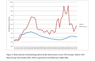
The graph shows that following widespread market reform at the end of the 20th Century there was big boom in investment in the two main natural gas technologies. More recently renewables have played an increasing role and there was a revival of investment in coal up to 2012. These trends are also partly driven by the lagged (because investment takes time) effects of fuel prices:

We find that electricity market deregulation resulted in significant immediate investment in various natural gas technologies, and a reduction in coal investments. However, market deregulation impacted less negatively on high efficiency coal technologies. In states that adopted wholesale electricity markets, high natural gas prices resulted in more investment in coal and renewable technologies.

There is also evidence that market liberalization encouraged investments into more efficient technologies. High efficiency coal technologies were less negatively affected by market
liberalization than less efficient coal technologies. Market liberalization also resulted in increased investment into high efficiency combined cycle gas. In summary the effect of liberalization is most negative for the least efficient coal technology and most positive for the most efficient natural gas technology.

The second paper is based on a survey of households in rural China and assesses the potential for energy conservation and carbon emissions mitigation when energy saving technologies are not fully implemented. In reality, appliances do not always survive for their designed lifetime and households often continue to use other older technologies alongside the new ones. The effect is to raise the cost of reducing energy use and emissions by a given amount. The paper computes marginal abatement cost curves under full and partial implementation of the new technologies.

The graph shows the marginal abatement cost curve for rural households in Hebei Province, scaled up from the survey and our analysis. Full-Scenario is the curve with full implementation of new technologies and OII-Scenario is with actual partial implementation. This analysis does not take into account any potential rebound effect of energy efficiency improvements.

The first author, Weishi Zhang, is a PhD student at the Chinese University of Hong Kong. She contacted me last year about possibly visiting ANU, and I supported her application for a scholarship to fund the visit (which unfortunately she didn't get), because I thought her research was some of the more interesting research on Chinese energy use and pollution that I had seen. I helped write the paper (and responses to referees in our revise and resubmit).